Conjugate Priors in R: The Shortcut That Gives Exact Posteriors Without MCMC
You ran a small test on your website. Nine visitors saw a new button. Six of them clicked. You want to know the true click-through rate, with an honest sense of how uncertain that estimate is. There is a one-line trick in R that gives you the answer exactly. No simulation, no integration, no extra packages. The trick has a name, conjugate priors, and once you understand it, you will reach for it for the rest of your career.
If 6 out of 9 visitors clicked, what's the true click rate?
Take a moment with this question, because it's stranger than it looks. The natural answer is "6 divided by 9, which is 67%." That's not wrong, exactly. It's the most likely rate given what you saw. But it hides something important.
Imagine you flipped a perfectly fair coin nine times. Half the time you'd get more than 4 or 5 heads, half the time fewer. Sometimes you'd get 6 heads, or 7, or even 8. Getting 6 heads from a fair coin happens about 16% of the time. So if a friend showed you 6 heads in 9 flips and said "this coin is biased toward heads," you'd be skeptical. The data is just not strong enough to support a confident claim.
Same principle here. With only 9 visitors, "6 clicked" doesn't pin down the true rate. Maybe the true rate is 50% and you got slightly lucky. Maybe it's 70% and you got slightly unlucky. Maybe it's exactly 67%. With nine data points, you cannot tell those apart.
So the right answer to "what's the true click rate" is not one number. It's a range of plausible rates, with some rates more believable than others. We want to compute that range honestly. The recipe below does it in two steps. First, it produces two summary numbers (let's call them parameter A and parameter B) that completely describe the answer. Second, it asks two questions of those summary numbers: "what's the most likely rate?" and "what range contains 95% of the plausibility?" Both questions become a single line of R each.
Walk through what those four operations did. The first two lines stored the experiment's data, 9 visitors and 6 clicks. The next two lines computed the two summary parameters, by starting from 1 (which represents "no opinion before the test", we'll explain shortly) and adding the data: clicks to parameter A, non-clicks (3 in this case) to parameter B. So post_a ended up at 7 and post_b at 4. The fifth code line, post_a / (post_a + post_b), is the formula for the most likely rate when you have these two summary parameters. It's just 7 / (7 + 4) = 7/11, which is 0.636. The last code line uses R's built-in qbeta() function to read off the 95% range from the same two parameters. The result is two numbers: the lower edge of the range and the upper edge.
Now the interpretation. The most plausible click-through rate is about 64%, slightly lower than the raw 6/9 = 67% because we started from "no opinion" rather than from "I trust the data exactly". There is a 95% chance that the true rate sits somewhere between 31% and 89%. Yes, that range is enormous, almost half of all possible rates. That's the honest answer when you have only 9 visitors. The data simply doesn't allow precision.
Notice that the variables post_a and post_b are the only numbers we needed to remember. From them, R's built-in functions can produce any range you want (qbeta) or any tail probability (pbeta). The two summary parameters carry all the information about the answer.
This is what the title of the post means by "shortcut." Most ways of computing this kind of answer require either calculus (integrating a complicated curve) or simulation (running thousands of random samples). For this kind of question, the shortcut is just adding two numbers and looking up the result.
qbeta(). Want the probability the rate exceeds 50%? Use 1 - pbeta(0.5, ...). The two parameters carry all the information about the answer.Try it: What happens if you ran a bigger experiment? Suppose 50 visitors saw the button and 32 clicked. Compute the same answer with that data. The most likely rate should stay close to 32/50 = 0.64. The 95% range should shrink because more data narrows uncertainty.
Click to reveal solution
The recipe was identical to before: start each parameter from 1, add clicks to A and non-clicks to B, divide for the most likely rate, use qbeta() for the 95% range. The only difference is the data values: A became 33 (1 + 32 clicks) and B became 19 (1 + 18 non-clicks).
The most likely rate is essentially unchanged at 0.63 (matching 32/50 = 0.64), but the 95% range tightened dramatically: from [0.31, 0.89] with 9 visitors down to [0.50, 0.76] with 50. More data sharpens the answer, exactly as it should.
What does the "1 +" in the formula represent?
You may have noticed something curious. The two key lines were post_a <- 1 + k and post_b <- 1 + (n - k). The data part makes sense (clicks and non-clicks), but where did those 1s come from? They are the answer to a deeper question: what did you believe about the click rate before you ran the test?
That belief, the one you had before seeing any data, is called a prior. The prior is just a starting position, a stance you take before the experiment begins. Even if you say "I have no opinion," that itself is a prior. It happens to be the prior we used in the previous section: every rate from 0% to 100% is equally believable. We encoded "no opinion" by setting both starting numbers to 1.
Here's the analogy that makes this concrete. Think of a weather forecaster the morning of a marathon. Before they look at any current data, they already have an expectation. "It's October in Chicago, so probably 50-something degrees, probably overcast, probably some rain." They haven't seen today's data, but they have a sensible starting point. That starting point is their prior. Then today's instruments report actual readings, and the forecaster updates the prior into a final forecast.
In our case, the "instruments" are the 9 visitors and 6 clicks. The "starting point" is the prior. The "final forecast" is the answer we computed. The two numbers post_a and post_b describe the final forecast. The two starting numbers, both 1, described our prior of "no opinion."
What if we'd had a different prior? Suppose, before running any test, you'd believed the click rate was probably around 20%, the typical rate for a new feature. You could encode that with prior_a = 2, prior_b = 8, which says "before seeing any data, my best guess is 2 clicks for every 10 visitors." The recipe stays the same: start from the prior numbers, add the data, look up the answer.
The code below tries three different priors on the same nine-visitor data. It uses a for loop to avoid repeating the same three lines for each prior. Each iteration prints the most likely rate and the 95% range under that prior.
Walk through what just happened. The list priors stored three labeled pairs of starting numbers: (1, 1) for "no opinion", (2, 8) for "I expected a low rate", and (8, 2) for "I expected a high rate". The loop pulled each pair, added the same data (6 clicks, 3 non-clicks) to each, and used the same formulas as before to get the most likely rate and the 95% range. The only thing that varied across the three iterations was the starting prior numbers; the data was identical.
Now the interpretation. The "no opinion" prior gave 0.64, basically the data itself. The "expected low" prior pulled the answer down to 0.47, because we told it "before the test, I really thought it was lower". The "expected high" prior pulled the answer up to 0.74. The data shifted each prior, but each starting position survived in the final answer.
Should this bother you? Not really. Two thoughts. First, every method of estimating things from data secretly involves a prior, even if the method doesn't admit it. The naive "6/9 = 67%" answer pretends there is no prior, but that is itself a stance: "I'm willing to act on raw data alone." Bayesian methods just make the prior explicit so you can examine it. Second, with enough data, the prior matters less and less. We'll see this in a moment. For now, just accept that the prior is part of the recipe, like flour in a cake.
Try it: Use a strong prior centered at 50%, encoded by prior_a = 50, prior_b = 50. With the 9 visitors and 6 clicks, what is the most likely rate? Notice how the strong prior anchors the answer near 50% even though the data leans toward 67%.
Click to reveal solution
The recipe was the same: start from the prior numbers (50 and 50), add the data (6 and 3), divide and look up. After the addition, parameter A was 56 and parameter B was 53.
The most likely rate landed at 0.51, almost exactly 50%. The strong prior dominated the small data because the prior contributed 100 hypothetical observations (50 for each side) while the data contributed only 9. The 95% range is also narrow for the same reason: with effectively 109 total observations, the answer is more confident than it would be with just the 9 real ones.
Why does this trick work?
You've now seen the recipe twice: take the prior, add the data, get the answer. It feels too simple. Where did all the math go? Did we accidentally skip something important? We didn't. The reason it really is this simple is worth understanding, because it tells you when the trick will and won't work in the future.
Here is an analogy. Imagine the Beta curve, which is the technical name for the family of curves the answer lives in, as a curve controlled by two dials. Dial A says "how many wins do you expect," dial B says "how many losses do you expect." Turn both dials up evenly and the curve gets taller and narrower around 50%. Turn dial A up alone and the curve shifts toward 100%. Turn dial B up alone and the curve shifts toward 0%. The shape can encode any belief about a rate.
Now consider what happens when you observe data. You saw 6 wins and 3 losses (out of 9 visitors). The simplest possible update is: turn dial A up by 6, turn dial B up by 3. That's exactly what post_a <- prior_a + k and post_b <- prior_b + (n - k) were doing in the code.
The mathematical lucky break is this: if you start with a Beta-shaped prior, and your data is a count of wins out of trials, then the only update you need to make to the curve is to turn the dials. The shape stays Beta. The curve doesn't morph into something weird that you'd need integrals to describe. It stays in the same family, just with the dials in new positions.
That is what "conjugate" means in this context. Two things are conjugate if they fit together algebraically so that combining them keeps the shape simple. The Beta curve and the binary-outcome data (clicks/no-clicks, wins/losses, yes/no) are conjugate. Most pairings of curve and data are not conjugate. When they are, you get the arithmetic shortcut. When they are not, you need a more powerful tool like MCMC.
So "conjugate priors" simply means: prior shapes that pair nicely with their data type, so the math reduces to addition. There are about half a dozen famous conjugate pairs, and three of them cover most everyday data analysis tasks. We'll see all three in the next section.
Try it: Confirm the "dial" analogy by drawing the curves. Plot a Beta curve with dials at 2 and 8, then a Beta curve with dials at 8 and 2. The first should peak near 0.2 (low rate), the second near 0.8 (high rate).
Click to reveal solution
The first line built a sequence of 200 candidate rates from 0 to 1 (so we have a smooth horizontal axis to plot against). The plot() call drew the first Beta curve (dials 2 and 8) using dbeta() to compute the density at each candidate rate. The lines() call overlaid the second Beta curve (dials 8 and 2) on the same axes. The legend() call labeled which is which.
You'll see the black curve peaks near 0.2 and the orange curve peaks near 0.8. Same family of curve, different dial positions, very different beliefs about the rate. This is what the dial analogy looks like in pictures.
Does this trick work for other kinds of data?
Yes, with three popular variants. Each one fits a different kind of data. The pattern is always the same: a prior shape with a small number of dials, a data type that fits algebraically, and an addition rule that combines them.
For yes/no data: Beta and Binomial
This is what you've been using. Yes/no data (clicks, conversions, wins, defects, survey yes-or-no answers) pairs with the Beta curve. Two dials. The update rule: add observed yeses to dial A, observed nos to dial B.
You have already seen this case. Skip ahead unless you want to read another example.
For count data: Gamma and Poisson
When you're counting events that happen at some unknown rate, like customer support tickets per day, accidents per month, server crashes per week, the right pair is the Gamma curve with Poisson data. The Gamma curve has two dials, like Beta did. You set the prior dials to encode your belief about the rate, observe some count data, and add.
Suppose your support team handled 8, 12, 7, 15, and 9 tickets across five days. Without strong prior knowledge, encode "around 8 tickets per day, but I'm not very sure" as Gamma(2, 0.25) (the two arguments are the prior dials). The update rule for Gamma-Poisson: add the total number of events observed to dial A, and add the number of observation periods to dial B.
Walk through the code. The first line stored the five days of ticket counts as a vector. The next two lines set the prior dials to 2 and 0.25 (encoding "I expect around 8 per day, but I'm not sure"). The two post_a and post_b lines applied the Gamma-Poisson update rule: sum(y) is the total events (51 across the 5 days), length(y) is the number of days (5). So post_a became 53 (2 + 51) and post_b became 5.25 (0.25 + 5). The last two lines asked the same kinds of questions as in the click-through case, but using qgamma() instead of qbeta() because we're working with rates, not proportions. The formula post_a / post_b is the most-likely-rate formula for the Gamma curve.
Interpretation: the most likely ticket rate is 10.1 per day, and there's a 95% chance the true rate is somewhere between 7.6 and 12.9 per day. The data nudged the prior up from "around 8" to "around 10" because the observed average (51/5 = 10.2) was higher than the prior centered at 8. The posterior also tightened because we contributed five real observations to the prior's prior weight of 0.25.
For Normal data with a known measurement spread: Normal and Normal
Now suppose your data is continuous measurements, like blood pressure readings, exam scores, or sensor outputs. If the readings are roughly bell-shaped (which most measurements are) and you happen to know the typical measurement spread (sigma), the prior shape is also Normal, and again we have a conjugate pair.
The arithmetic here is slightly more involved than just adding numbers. Each of the prior and the data has a confidence, which is just one over the variance. The posterior mean is a weighted average of the prior mean and the data mean, weighted by their confidences. More data = higher data confidence = data wins. Stronger prior (lower prior sd) = higher prior confidence = prior wins.
Walk through what the code did. The first three lines stored the ten readings, the count of readings (10), and the known measurement spread sigma = 10. The next two lines stored the prior: a Normal curve centered at 120 with spread 8. The two _prec lines computed the prior and data confidences as 1 / variance. The prior confidence is 1 / 8^2 = 0.0156. The data confidence is 10 / 10^2 = 0.10. So the data is about 6.4 times more confident than the prior. The post_var line combined the two confidences (just by adding them) and inverted to get the posterior variance. The post_mean line is the precision-weighted average: each side of the average (prior_mean and data mean) contributes in proportion to its confidence. The last qnorm() line asks the same 95%-range question as before, using the Normal curve.
Interpretation: the most likely underlying mean is 125.7, and the 95% range is [121.4, 130.0]. The data mean was 128.8, the prior mean was 120, and the answer landed at 125.7, much closer to the data because the data carried 6.4x the confidence of the prior. If the prior had been stronger (smaller prior_sd), the answer would have leaned closer to 120.
You can stop the survey here. Three pairs cover most everyday work: Beta-Binomial for yes/no, Gamma-Poisson for counts, Normal-Normal for measurements. They are all in R's base distribution functions. No package install needed.
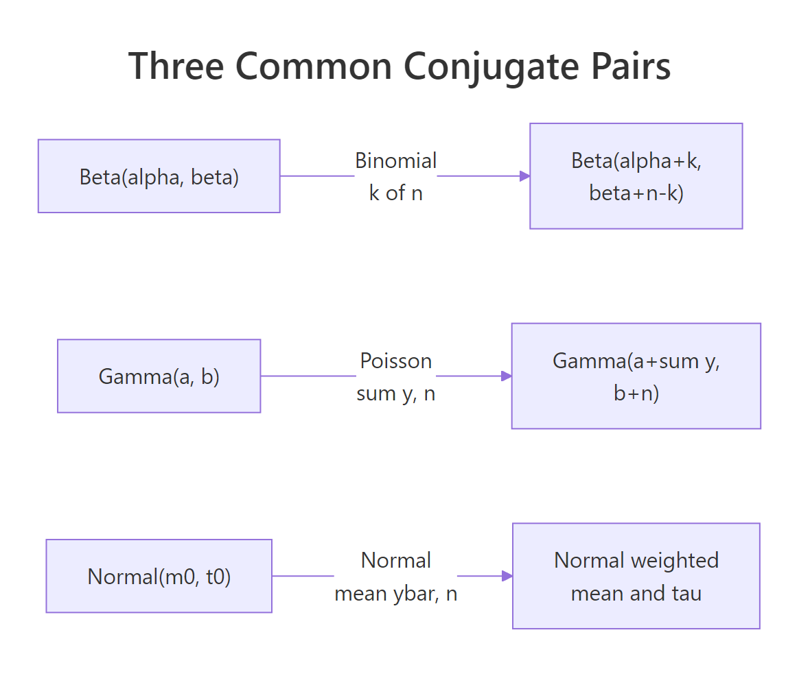
Figure 1: The three common conjugate pairs and the closed-form parameters of the posterior in each case.
qbeta, qgamma, qnorm) away.Try it: Suppose you observed 25 emergency calls in 4 hours and want a posterior on calls per hour. Use a Gamma(1, 0.5) prior (mild belief in low rates). Compute the most likely rate and the 95% range.
Click to reveal solution
The recipe was the same as the support-tickets case: add total events (25 calls) to dial A, add observation periods (4 hours) to dial B. So post_a became 26 and post_b became 4.5. The most-likely-rate formula post_a / post_b gave 5.78. The qgamma() call gave the 95% range.
The most likely rate is 5.8 calls per hour, with a 95% range of [3.8, 8.1]. Same pattern as before, just with qgamma() instead of qbeta() because the data was counts instead of yes/no.
What if I picked the wrong prior?
This is the worry that prevents many people from using Bayesian methods at all. They think: "if my answer depends on a prior I made up, isn't the answer just my own bias dressed up as math?" It's a fair worry. The answer is: yes, with little data, but no, with enough data. And there is a clean way to check.
The check is to try several priors that a reasonable analyst could plausibly have chosen, and see how much the final answer moves. If three reasonable priors give nearly the same answer, the conclusion is robust, your prior didn't really matter. If they give very different answers, that's itself a finding: "with this little data, the conclusion depends on the starting point. We need more data to be confident."
Back to the click-through example. Nine visitors, six clicks. The code below loops over three different priors that bracket what a reasonable analyst might pick, and for each, applies the same Beta-Binomial update we've been using.
Walk through the code. The list priors stored three labeled pairs of dial values. The loop pulled each pair into p, applied the Beta-Binomial update (pa = first dial + 6 clicks, pb = second dial + 3 non-clicks), then computed the most likely rate and the 95% range as in earlier sections. cat(sprintf(...)) is just a formatting trick to print one line per prior with aligned columns.
Now the interpretation. Three priors gave three quite different answers, even though the data was identical. The skeptical prior pulled the rate down to 0.50, the flat prior left it near the data at 0.64, the optimistic prior pulled it up to 0.78. With nine visitors, the prior matters, a lot.
Now suppose we collected more data: 50 visitors, 32 clicks. The same loop, just with bigger numbers in the data part of the update.
The code is structurally identical to the previous one, just using n2 and k2 (the bigger experiment's numbers) where the previous used 9 and 6. The result is one line per prior showing the most likely rate.
Look at the difference. With nine visitors, the three priors gave answers from 0.50 to 0.78, a range of 0.28. With fifty visitors, the same three priors give answers from 0.60 to 0.67, a range of just 0.07. Same priors, far less disagreement, because the data swamps the prior with enough evidence. With 500 visitors, the three answers would be within 1% of each other. With 5,000, they'd be indistinguishable.
That's the answer to "what if I picked a bad prior?" If you have enough data, the prior didn't matter. If you didn't have enough data, the prior did matter, and the right thing to do is report all three answers and let the reader decide. That's what makes Bayesian analysis honest: the assumptions are visible, the sensitivity is testable, and the result is not falsely precise when the data doesn't support precision.
Try it: Repeat the sensitivity check with the bigger experiment (50 visitors, 32 clicks) but using stronger priors: c(20, 50), c(10, 10), c(80, 20). Even with more data, very strong priors can dominate. See if you can find a prior strong enough to still matter.
Click to reveal solution
The loop did exactly what it did before, but the prior dial values were much larger this time. For example, the strong skeptical prior added 20 to dial A (instead of 2), so even after the data added 32 clicks, the prior was still contributing a substantial chunk.
Even with 50 data points, the very strong priors (worth 70 to 100 hypothetical observations) pulled the answer noticeably. The strong skeptical prior pulled all the way down to 0.45, the strong optimistic pushed up to 0.70. This is why prior choice matters and why you report sensitivity: a strong prior plus modest data can move the answer by 0.25.
When does this trick stop working?
The arithmetic of conjugate priors is gorgeous when it works. But the list of pairs that are conjugate is short, and the moment your problem leaves that list, the arithmetic disappears and you need a different tool.
Three places this happens.
First, when there are two unknowns instead of one. The Normal-Normal example we did earlier assumed we knew the measurement spread (sigma). What if we don't? Now the unknowns are the underlying mean and the underlying spread. There is a more elaborate conjugate pair for that case, but it's noticeably uglier than the cases we've seen, and the moment you have a third unknown the elegance is gone.
Second, in hierarchical models. Suppose you have customer data from 50 different stores, and you want to estimate a per-store conversion rate while also estimating an overall company average. The store rates inform the company rate, the company rate informs the store rates. The math no longer factors into a single addition step. You need iterative methods.
Third, when your data shape doesn't match a standard distribution. Maybe your outcome is a positive number with a long right tail, or counts that are zero-inflated, or some custom thing you defined for your business. Off the conjugate list, the addition trick doesn't apply.
In all three cases, the standard tool is MCMC, which stands for Markov Chain Monte Carlo. The names and acronyms are unimportant. What matters is that MCMC computes the same kind of answer (most likely value, 95% range, probability of an event) but instead of doing it with arithmetic, it does it by drawing a large number of random samples from the posterior. The R packages brms and rstan make MCMC accessible without writing the sampling code yourself.
Here's a small demonstration of why MCMC takes over when there are too many unknowns. Suppose we wanted to fit the Normal model with both mean and spread unknown. We could try to brute-force it by laying down a grid of (mean, spread) pairs and scoring each one against the data. With 80 candidate means and 80 candidate spreads, that's 6,400 cells, totally fine. With 5 unknown parameters at 50 candidates each, it's 312 million cells. The cost grows exponentially with the number of unknowns, and that's exactly the wall MCMC was invented to scale past.
Walk through the code. The first two lines created 20 simulated measurements from a Normal distribution with true mean 5 and true spread 1.5, so we know the ground truth and can check the answer. The next two lines built two grids: 80 candidate values of the unknown mean (between 3 and 7), and 80 candidate values of the unknown spread (between 0.5 and 3). The outer() function combines them into all 80 × 80 = 6,400 (mean, spread) pairs and scores each pair against the observed data, using the log-likelihood for numerical stability. The next line normalized the scores into probabilities (dividing by their total). The last line collapsed the 2D table down to a 1D summary by averaging over the spread dimension, giving the most likely value of the unknown mean.
Interpretation: the most likely mean came out to 5.12, very close to the true value of 5. The brute-force grid worked fine for 6,400 cells. But add a third unknown at the same resolution and you'd be at 512,000 cells. A fifth and you'd be in the hundreds of millions. Real Bayesian models often have dozens of parameters, and that's the wall MCMC was invented to scale past.
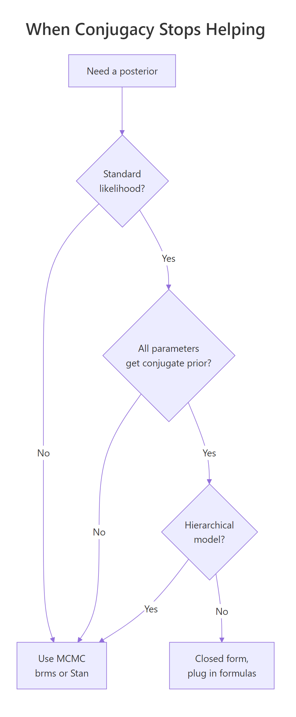
Figure 2: When conjugacy stops helping. Most realistic models fall off this tree quickly.
Try it: Roughly how many cells does a brute-force grid need for 5 unknown parameters at 50 candidates each? This is the comparison that motivates moving to MCMC.
Click to reveal solution
The expression 50 ^ 5 is just 50 to the fifth power, since for each of the 5 unknowns we have 50 candidate values, and we need every combination.
The result is over 312 million cells, each requiring a likelihood evaluation. Even at fast speeds this is hours of compute. By 7 unknowns it's centuries. That's the practical wall MCMC was invented to scale past.
Practice Exercises
Exercise 1: A click-through rate from a small ad
A new ad got 8 clicks out of 50 impressions. Use a Beta(2, 8) prior (mildly skeptical, mean of 0.20). Report the most likely rate, the 95% range, and the posterior probability that the true rate exceeds 5%.
Click to reveal solution
The Beta-Binomial update added 8 clicks to dial A (so post_a = 10) and 42 non-clicks to dial B (so post_b = 50). The most-likely-rate formula post_a / (post_a + post_b) gave 10/60 = 0.167. qbeta() gave the 95% range. 1 - pbeta(0.05, ...) is "1 minus the chance the rate is below 5%", which is the chance the rate is above 5%.
Most likely rate: 17%. 95% range: [8%, 28%]. Probability the true rate exceeds 5%: about 99%. Strong evidence the ad outperforms a 5% threshold.
Exercise 2: An A/B test using two posteriors at once
This exercise teaches a small superpower of Bayesian posteriors. Once you have the two summary parameters, you can also draw random samples from the posterior using rbeta(). And once you have draws from two posteriors, you can compare them directly to answer questions like "what's the probability variant B beats variant A?"
Variant A got 84 clicks from 1,200 impressions. Variant B got 105 clicks from 1,180 impressions. Use a flat Beta(1, 1) prior on each. Use the closed-form posteriors to draw 100,000 samples from each, and report the probability that B's true rate is higher than A's.
Click to reveal solution
The first two lines computed each variant's posterior parameters with the standard Beta-Binomial update. set.seed(2026) made the random sampling reproducible. The two rbeta() calls each drew 100,000 samples from one of the posterior curves. The last line compared the two sample vectors element-by-element (b_draws > a_draws produces a vector of TRUE/FALSE) and computed the proportion that were TRUE, which is the probability B's rate exceeds A's.
About 97% probability that B's true rate is higher than A's. That's a clean answer to give to a stakeholder, no need to translate from p-values or talk about null hypotheses.
Exercise 3: A blood-pressure mean from prior and data
Five blood-pressure readings: 132, 128, 135, 121, 138. Known measurement standard deviation: 8. Prior on the underlying mean: Normal(120, 10). Compute the most likely underlying mean and the 95% range.
Click to reveal solution
The recipe is the Normal-Normal update from the main text. Prior confidence (prior_prec) is one over prior_sd squared. Data confidence (data_prec) is the count of readings divided by sigma squared. The posterior variance is one over the sum of the two confidences, and the posterior mean is the precision-weighted average of the prior mean (120) and the data mean (130.8).
Most likely underlying mean: 128.7. 95% range: [122.0, 135.5]. The data mean was 130.8, the prior mean was 120, and the answer landed at 128.7, much closer to the data because five measurements with sigma = 8 carry more weight than a prior with sd = 10.
Complete Example: A Customer Satisfaction Report
A SaaS company surveys 200 customers. 132 say they would recommend the product. Marketing wants to claim the recommendation rate is "above 60%." Quantify that claim under three priors (skeptical, flat, optimistic) and report whether the conclusion is robust to prior choice.
Walk through the code. The data was 200 surveys with 132 yeses. The list priors defined three different starting beliefs. The loop applied the Beta-Binomial update under each prior (pa = first dial + 132, pb = second dial + 68), then computed three quantities: the most likely rate, the 95% range, and the probability the true rate is above 60% (computed as 1 - pbeta(0.60, ...), the chance of being above 0.60 rather than below). Results are printed one row per prior with aligned columns.
Interpretation: all three priors give a most-likely rate within 0.02 of each other (0.65 to 0.67), and all three give a posterior probability above 90% that the true rate exceeds 60%. Marketing's claim is robust: under three reasonable starting beliefs, the data strongly support "the rate is above 60%." That's the kind of confident, honest answer you can hand to a stakeholder, plus the sensitivity check that demonstrates you didn't cherry-pick the prior. Eight lines of base R, no packages.
Summary
The shortcut works whenever your prior shape and your data type are conjugate. Three pairings cover most everyday data analysis:
| Type of data | Prior shape | Update rule (closed-form posterior) |
|---|---|---|
| Yes/No (proportions) | Beta(a, b) | Beta(a + clicks, b + non-clicks) |
| Counts (rates) | Gamma(a, b) | Gamma(a + total events, b + observation periods) |
| Normal data with known spread (means) | Normal(m, s) | Precision-weighted mix of m and the data mean |
In each case, R has a built-in function (qbeta, qgamma, qnorm) that turns the two posterior parameters into ranges and probabilities. No extra packages, no MCMC, no integration.
When you can use the shortcut, do. When you cannot (more than two unknowns, hierarchical models, custom data shapes), reach for brms or rstan and let MCMC do the work. The mental model, prior plus data give an updated belief, is the same in both worlds.
References
- Johnson, A. A., Ott, M. Q., Dogucu, M. Bayes Rules! An Introduction to Applied Bayesian Modeling, Chapman & Hall, 2022. Chapter 5 covers conjugate families with worked R code. Open access at bayesrulesbook.com/chapter-5.
- Gelman, A., Carlin, J. B., Stern, H. S. et al. Bayesian Data Analysis, 3rd ed., Chapman & Hall, 2013. Chapters 2-3 derive the standard conjugate families.
- Cook, J. D. "Diagram of Bayesian conjugate priors." johndcook.com/blog/conjugate_prior_diagram. Interactive cross-family reference.
- Fink, D. "A Compendium of Conjugate Priors." 1997. johndcook.com/CompendiumOfConjugatePriors.pdf. Comprehensive table of conjugate pairings.
- Gelman, A. and the Stan team. "Prior choice recommendations." github.com/stan-dev/stan/wiki/Prior-Choice-Recommendations. The community standard reference for principled prior selection.
- CRAN Task View: Bayesian Inference. cran.r-project.org/web/views/Bayesian.html. Curated list of Bayesian R packages.
Continue Learning
- Bayesian Statistics in R, the section opener that walks through the prior-data-posterior workflow with simulation and visualization, building the intuition that conjugacy then turbocharges.
- Grid Approximation in R, what to do when the conjugate shortcut does not apply but you still want a posterior in base R, no MCMC required.
- Bayes' Theorem in R, the discrete starting point worked through a medical-test example, ideal background reading if anything in this post still feels abstract.