ARFIMA in R: Long-Memory Models with fracdiff
ARFIMA (AutoRegressive Fractionally Integrated Moving Average) is an ARIMA model whose differencing order d is allowed to be a fraction instead of a whole number. That single change lets it capture long memory: series whose autocorrelation fades so slowly that a standard ARIMA cannot describe it. In R you fit one with the fracdiff package.
What is long memory, and why does ARIMA miss it?
You already know ARIMA's d as a whole number: d = 0 for a stationary series, d = 1 when you difference once to kill a trend, d = 2 for a doubly-integrated series. Long memory lives in the gap between those integers. Some real series, river levels, inflation, market volatility, network traffic, are not a random walk (d = 1), yet their shocks fade far too slowly for a short-memory model (d = 0). The clearest fingerprint is the autocorrelation function (ACF). Let's compare the exact ACF of a long-memory process against a short-memory AR(1) and watch the difference.
For an ARFIMA(0, d, 0) process there is a closed-form autocorrelation at every lag, so we can compute it directly instead of simulating. We put it next to an AR(1) whose autocorrelation is simply the coefficient raised to the lag power.
Read across the two bottom rows. Both processes start near 0.6 at lag 1, so at first glance they look similar. But by lag 10 the AR(1) has all but forgotten its past (autocorrelation 0.006), while the long-memory process is still strongly correlated at 0.42. At lag 100 the AR(1) autocorrelation is effectively zero, yet the long-memory process is still at 0.27. That very slow decay is exactly what "long memory" means.
The reason ARIMA cannot capture this is structural. A short-memory ACF decays geometrically, like 0.6^k, which drops to nothing within a handful of lags. A long-memory ACF decays much more slowly, at a hyperbolic (power-law) rate. In symbols, its tail behaves like this:
$$\rho_k \sim c \, k^{2d - 1} \quad \text{as } k \to \infty$$
Where $\rho_k$ is the autocorrelation at lag $k$, $c$ is a constant, and $d$ is the fractional differencing order. Because $2d - 1$ is negative for $d < 0.5$, the autocorrelation shrinks, but as a slow power of $k$ rather than a fast exponential. If you are not interested in the math, skip it: the practical point is in the table above.
d is built to model.Try it: Weaker long memory means a smaller d. Use the arfima_acf() function above to compute the lag-50 autocorrelation for d = 0.2 and see how much lower it is than the d = 0.4 value of 0.307.
Click to reveal solution
Explanation: With d = 0.2 the lag-50 autocorrelation is 0.0243, far below the 0.307 we saw at d = 0.4. The memory is still longer than an AR(1) would give, but a smaller d means the past fades faster.
What does the "d" in ARFIMA(p, d, q) actually mean?
Ordinary differencing is the operation y_t - y_{t-1}. Written with the lag operator L (which just means "shift back one step", so L y_t = y_{t-1}), that is (1 - L) y_t. Differencing twice is (1 - L)^2. ARIMA only ever raises (1 - L) to a whole-number power. Fractional differencing asks a bolder question: what if the exponent could be any real number, like 0.4?
The answer comes from the binomial series, which expands (1 - L)^d into an infinite sum of lag terms:
$$(1 - L)^d = \sum_{k=0}^{\infty} \binom{d}{k} (-L)^k$$
Where $L$ is the lag operator, $d$ is the (possibly fractional) differencing order, and $\binom{d}{k}$ is the generalized binomial coefficient. You never compute that by hand, because the coefficients follow a simple recursion: start at 1, then multiply by (k - 1 - d) / k for each new term. Let's turn that recursion into a function and look at the weights for d = 0.4.
These eight numbers are the recipe for fractional differencing. To fractionally difference a series, you take today's value with weight 1, subtract 0.4 times yesterday, subtract 0.12 times the day before, and so on down a slowly shrinking tail. Every past value contributes a little. Now compare that to ordinary first differencing, which is the same operator with d = 1.
Ordinary differencing keeps only two nonzero weights: weight 1 on today, weight -1 on yesterday, and exactly zero on everything older. It only ever looks one step back. Fractional differencing keeps a long, fading tail of weights instead, which is precisely how it removes long memory without throwing away the slow structure the way a full first difference would.
This also explains where d sits on a spectrum. At d = 0 there is no differencing at all (a short-memory ARMA series). As d grows toward 1 you approach a random walk. The interesting territory is in between.
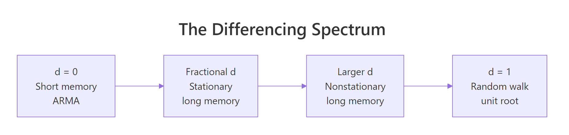
Figure 1: The differencing spectrum. ARFIMA fills the gap between d = 0 (short memory) and d = 1 (a random walk); a fractional d between 0 and 0.5 gives a stationary long-memory process, while d from 0.5 up to 1 is long memory that is no longer stationary.
Try it: Generate the first 6 fractional differencing weights for d = 0.5 with the diff_weights() function. The weights for a larger d fall off faster; notice which one first drops below 0.05 in size.
Click to reveal solution
Explanation: The first weight is always 1. The second is -d, here -0.5. From the fifth weight on (-0.0391) the values are below 0.05 in size, so a larger d still keeps a tail but that tail thins out faster than the d = 0.4 case.
How do you simulate a long-memory series in R?
Fractional differencing has a mirror image called fractional integration, written (1 - L)^(-d). Where differencing strips memory out, integration builds it in: it turns plain white noise into a long-memory series. The weights come from the same recursion with a flipped sign, so let's look at them for d = 0.4.
Read these as an echo. A shock that hits the series today still contributes 0.14 of its size seven steps later, and the tail keeps going. That lingering influence is the mechanism behind long memory. To actually build a long-memory series, we filter a stream of random shocks through these weights.
Those are the sample autocorrelations at lags 1, 2, 5, 10, 20, and 40. They start high and come down, but slowly: even 40 steps back the series is still correlated at 0.204. A short-memory series would have hit zero long before lag 40. We built genuine long memory out of nothing but random noise and a set of fading weights.
fracdiff.sim() function that generates the same kind of series in one call, and it can add AR and MA terms too. The manual version above is here to show what is happening under the hood.Here is the package doing it directly. This block, and every other block that uses the fracdiff package, is meant to run in your local R session (RStudio or the R console), not in the browser.
library(fracdiff)
set.seed(2026)
ym <- fracdiff.sim(n = 2000, ar = numeric(0), ma = numeric(0), d = 0.4)$series
round(head(ym, 6), 4)
#> [1]  0.7490 -0.6585  0.0026 -0.0845 -0.7012 -2.8553
The $series element holds the simulated values (the function also returns the settings you gave it). We now have a 2000-point series ym with a known true d of 0.4, which is the perfect test case for estimating d back from data in the next section.
Try it: Use the base-R int_weights() function to simulate a weaker long-memory series with d = 0.25 and n = 1000, then look at its autocorrelation at lags 1, 5, and 10. A smaller d should give faster decay.
Click to reveal solution
Explanation: With d = 0.25 the lag-1 autocorrelation is 0.287 and it decays to 0.058 by lag 10, much faster than the d = 0.4 series but still slower than a short-memory process would.
How do you estimate d with the fracdiff package?
Simulating is the easy direction. The real job is the reverse: given a series, estimate d. The fracdiff package does this by maximum likelihood, which searches for the d that makes the observed data most probable. We call fracdiff() on our simulated series and ask for zero AR and zero MA terms, since we know it is a pure ARFIMA(0, d, 0).
fit <- fracdiff(ym, nar = 0, nma = 0)
round(fit$d, 4)
#> [1] 0.3987
summary(fit)
#>
#> Call:
#>   fracdiff(x = ym, nar = 0, nma = 0)
#>
#> Coefficients:
#>    Estimate Std. Error z value Pr(>|z|)
#> d 3.987e-01  2.945e-05   13539   <2e-16 ***
#> sigma[eps] = 0.9779956
#> Log likelihood: -2794 ==> AIC = 5592.108 [2 deg.freedom]
The estimate is fit$d = 0.3987, almost exactly the true value of 0.4. The summary() output adds the sort of table you expect from a regression: an estimate, a standard error, a z value, and a p-value, plus the residual standard deviation sigma[eps] and an AIC for model comparison. On the surface, d looks extraordinarily precise.
fit$d as a good point estimate, but get your sense of uncertainty from a second method.That second method is a semiparametric estimator, which reads d off the shape of the series' spectrum (a frequency-based view of the series) rather than assuming a full model. The fracdiff package offers two: fdGPH() (the Geweke and Porter-Hudak estimator) and fdSperio() (a refinement by Reisen). Running both alongside the maximum-likelihood estimate gives you an honest spread.
gph  <- fdGPH(ym)      # Geweke and Porter-Hudak
sper <- fdSperio(ym)   # Reisen
round(c(MLE = fit$d, GPH = gph$d, Sperio = sper$d), 4)
#>    MLE    GPH Sperio
#> 0.3987 0.4811 0.3623
The three estimates, 0.399, 0.481, and 0.362, straddle the true 0.4. That range is the real uncertainty in d, and it is far wider than the maximum-likelihood standard error suggested. When you report an ARFIMA fit, quoting all three numbers is more honest than quoting fit$d alone.
Try it: The estimated d is stored in fit$d. Print it rounded to 3 decimals so you have the value to two more digits than the summary table shows.
# The fitted model object is called `fit`.
# Pull out fit$d and round it to 3 decimal places.
# your code here
Click to reveal solution
round(fit$d, 3)
#> [1] 0.399
Explanation: fit$d holds the maximum-likelihood estimate, 0.399, which rounds cleanly from the 0.3987 we saw earlier. Storing model results in a named object and pulling pieces out with $ is the standard way to reuse a fit.
How do you undo long memory with fractional differencing?
Estimating d is only useful if you do something with it. The classic move is to fractionally difference the series by its own d, which strips out the long memory and leaves a short-memory series you can model with an ordinary ARMA. Let's first prove the idea with our base-R weights on the hand-built series y, then use the package function on ym.
Compare this to the raw series, which had autocorrelations of 0.568 down to 0.204 across the same lags. After fractional differencing, every autocorrelation sits near zero: this is white noise. The long memory is gone. The package does the exact same thing with diffseries(), which takes the series and a value of d and applies the fractional-differencing filter for you.
ym_d <- diffseries(ym, d = fit$d)   # use the estimated d
before <- round(acf(ym,   plot = FALSE, lag.max = 50)$acf[c(2, 11, 26, 51)], 3)
after  <- round(acf(ym_d, plot = FALSE, lag.max = 50)$acf[c(2, 11, 26, 51)], 3)
rbind(lag = c(1, 10, 25, 50), before = before, after = after)
#>         [,1]   [,2]   [,3]   [,4]
#> lag    1.000 10.000 25.000 50.000
#> before 0.572  0.239  0.171  0.127
#> after  0.010  0.001  0.013  0.009
The before-and-after table tells the whole story. Before differencing, the series is still correlated at 0.127 fifty lags back. After differencing by the estimated d, the autocorrelations collapse to near zero at every lag. You have separated the long-memory component (captured by d) from the short-memory dynamics (whatever is left in ym_d).
d soaks up the slow, long-range structure that would otherwise wreck an ARMA fit. Once you difference it out, the leftover series is short-memory and easy to model the ordinary way.Try it: What happens if you difference by too much? Use diffseries() to fractionally difference ym with d = 0.8, well above the true 0.4, then look at the lag-1 autocorrelation. A negative value is the classic sign of over-differencing.
# diffseries(x, d) applies fractional differencing.
# Difference ym with d = 0.8, then print the lag-1 autocorrelation rounded to 3 decimals.
# your code here
Click to reveal solution
ex_over <- diffseries(ym, d = 0.8)
round(acf(ex_over, plot = FALSE, lag.max = 1)$acf[2], 3)
#> [1] -0.275
Explanation: Differencing by 0.8 when the true d is 0.4 removes too much, and the series swings the other way into negative correlation (-0.275 at lag 1). Matching d to the data, not overshooting it, is what leaves clean white noise behind.
How do you forecast a long-memory series?
The payoff of fitting an ARFIMA model is forecasting, and long memory changes the shape of a forecast in a way worth seeing. The forecast package knows how to forecast a fracdiff object directly, so we hand it our fitted model and ask for eight steps ahead.
library(forecast)
fc <- forecast(fit, h = 8)   # fit and ym are already in memory
round(as.data.frame(fc), 4)
#>      Point Forecast   Lo 80  Hi 80   Lo 95  Hi 95
#> 2001        -0.5795 -1.8336 0.6745 -2.4974 1.3384
#> 2002        -0.5929 -1.9430 0.7571 -2.6577 1.4718
#> 2003        -0.5830 -1.9776 0.8116 -2.7158 1.5499
#> 2004        -0.5691 -1.9914 0.8533 -2.7444 1.6062
#> 2005        -0.5553 -1.9974 0.8867 -2.7607 1.6501
#> 2006        -0.5426 -1.9997 0.9145 -2.7711 1.6859
#> 2007        -0.5311 -2.0003 0.9381 -2.7780 1.7158
#> 2008        -0.5207 -1.9999 0.9585 -2.7830 1.7415
Look at the point forecasts drifting from -0.58 back toward -0.52 over eight steps. The series mean is about -0.05, so eight steps out the forecast has barely started returning to it. That is the signature of long memory: forecasts revert to the mean slowly, and the prediction intervals (the Lo and Hi columns) widen slowly too, because the distant past still carries information about the future. A short-memory AR model would have snapped back to the mean within a few steps.
forecast::arfima() will estimate d together with the AR and MA orders automatically, then you forecast the result the same way. It is the one-call convenience wrapper around the fracdiff machinery.Try it: Forecast 12 steps ahead instead of 8 and compare the last point forecast to the series mean, mean(ym). How far apart are they still?
# fit and ym are already in memory.
# Forecast 12 steps ahead, then compare the last point forecast to mean(ym).
# your code here
Click to reveal solution
ex_fc <- forecast(fit, h = 12)
round(c(last_forecast = tail(ex_fc$mean, 1), series_mean = mean(ym)), 4)
#> last_forecast   series_mean
#>        -0.488        -0.046
Explanation: Even 12 steps out the forecast (-0.488) is nowhere near the series mean (-0.046). A long-memory process pulls back to its average at a crawl, which is why ARFIMA forecasts stay informative much farther into the future than short-memory ones.
Practice Exercises
These capstone problems combine several steps from the tutorial. Each solution runs in your local R session. Try them before opening the solutions.
Exercise 1: A full ARFIMA workflow from scratch
Simulate a fresh long-memory series with fracdiff.sim() using n = 1500 and d = 0.3. Estimate d two ways (maximum likelihood with fracdiff() and the GPH estimator with fdGPH()), then fractionally difference the series by the estimated d with diffseries() and confirm the result is white noise by checking the lag-1 autocorrelation of both the raw and the differenced series.
# 1. set.seed(321), then simulate with fracdiff.sim(n = 1500, d = 0.3)
# 2. estimate d with fracdiff() and with fdGPH()
# 3. difference with diffseries() using the MLE estimate
# 4. print the lag-1 ACF of the raw series and of the differenced series
# your code here
Click to reveal solution
set.seed(321)
cap_y   <- fracdiff.sim(n = 1500, d = 0.3)$series
cap_fit <- fracdiff(cap_y, nar = 0, nma = 0)
cap_wn  <- diffseries(cap_y, d = cap_fit$d)
round(c(mle_d    = cap_fit$d,
        gph_d    = fdGPH(cap_y)$d,
        raw_acf1 = acf(cap_y,  plot = FALSE)$acf[2],
        wn_acf1  = acf(cap_wn, plot = FALSE)$acf[2]), 4)
#>    mle_d    gph_d raw_acf1  wn_acf1
#>   0.2828   0.2766   0.3738   0.0048
Explanation: Both estimators land near the true 0.3 (0.283 and 0.277). The raw series has a clear lag-1 autocorrelation of 0.374, and after differencing by the estimated d it drops to 0.005, essentially white noise. That end-to-end path, simulate, estimate, difference, verify, is the core ARFIMA workflow.
Exercise 2: Does ARFIMA actually beat AR(1) here?
Using the simulated series ym from the tutorial, compare an ARFIMA(0, d, 0) fit against a plain AR(1) fit with arima(ym, order = c(1, 0, 0)) by their AIC values (lower is better). The ARFIMA AIC is -2 * fit$log.likelihood + 2 * 2 because the model spends two parameters. Which model does the data prefer?
# ARFIMA AIC: -2 * fit$log.likelihood + 2 * 2
# AR(1) AIC:  AIC(arima(ym, order = c(1, 0, 0)))
# print both, rounded to 2 decimals
# your code here
Click to reveal solution
aic_arfima <- -2 * fit$log.likelihood + 2 * 2
aic_ar1    <- AIC(arima(ym, order = c(1, 0, 0)))
round(c(ARFIMA = aic_arfima, AR1 = aic_ar1), 2)
#>  ARFIMA     AR1
#> 5592.11 5746.82
Explanation: The ARFIMA AIC (5592.11) is about 155 points below the AR(1) AIC (5746.82), a large gap. Because the data really does have long memory, the fractional model describes it far better than an AR(1) that can only see a few lags back. On a genuinely short-memory series the verdict would flip.
Exercise 3: Write your own fractional-difference function
The diffseries() function is convenient, but the operation is just the weighted sum you have already seen. Write a function my_fracdiff(x, d) that mean-centers the series, builds the differencing weights with diff_weights(), applies them with filter(), and drops the warm-up NA values. Confirm it produces near-white-noise by checking the lag-1 autocorrelation on ym with d = 0.4.
# diff_weights(d, n) is defined earlier in the tutorial.
# 1. mean-center x
# 2. build ~200 differencing weights
# 3. apply with filter(..., method = "convolution", sides = 1)
# 4. drop NA values, then print the lag-1 ACF
# your code here
Click to reveal solution
my_fracdiff <- function(x, d, trunc = 200) {
  z <- x - mean(x)
  w <- diff_weights(d, trunc)
  out <- as.numeric(filter(z, w, method = "convolution", sides = 1))
  out[!is.na(out)]
}
cap3 <- my_fracdiff(ym, 0.4)
round(acf(cap3, plot = FALSE, lag.max = 1)$acf[2], 3)
#> [1] 0.018
Explanation: Your hand-built function reduces the lag-1 autocorrelation of ym to 0.018, matching what diffseries() achieves. Truncating the weights at 200 lags keeps the filter fast while still capturing the memory; the small residual autocorrelation comes from that truncation and the finite sample.
Frequently Asked Questions
What range of d should I expect, and what does each value signal? For a stationary long-memory series, d falls between 0 and 0.5. Values from 0.5 up to 1 still show long memory but are no longer stationary, and d = 0 means no long memory at all (a plain ARMA series). Negative d down to -0.5 is possible too and signals "anti-persistence", where the series tends to reverse itself.
How is ARFIMA different from ARIMA? They are the same model except for the differencing order. ARIMA forces d to be a whole number (0, 1, 2), so it can only remove trends in coarse, integer steps. ARFIMA lets d be a fraction, which is the only way to capture the slow, hyperbolic autocorrelation decay that defines long memory.
How much data do I need to estimate d reliably? Long memory is a property of the far tail of the autocorrelation, so short series make d hard to pin down. The examples here use 1500 to 2000 points and recover d well. With only a few hundred observations, expect the maximum-likelihood and semiparametric estimates to disagree more, which is exactly why cross-checking with fdGPH() and fdSperio() matters.
Should I use the fracdiff package or forecast::arfima()? They are the same engine. Use fracdiff() directly when you want full control over the model and access to the estimation internals. Use forecast::arfima() when you want the AR, MA, and d orders chosen for you and a forecast object ready to plot. The convenience wrapper calls fracdiff underneath.
Can I combine long memory with AR and MA terms? Yes. That is the general ARFIMA(p, d, q) model. Pass nar and nma to fracdiff() (or let forecast::arfima() select them) to add short-memory AR and MA dynamics on top of the fractional differencing, which handles both the slow long-range structure and the quick local structure in one model.
Summary
ARFIMA generalizes ARIMA by letting the differencing order d be a fraction, which is what lets it model long memory: autocorrelation that fades too slowly for any integer-d model to describe.
| Idea | What to remember |
|---|---|
| Long memory | Autocorrelation decays as a slow power of the lag, not a fast exponential, so shocks persist for a long time |
The d parameter |
0 to 0.5 is stationary long memory; 0.5 to 1 is nonstationary long memory; 0 is short memory; 1 is a random walk |
| Fractional differencing | The operator (1 - L)^d expands into a slowly fading tail of weights that touches the whole past, unlike (1 - L) which only touches yesterday |
fracdiff() |
Estimates d by maximum likelihood; the point estimate is good but its standard errors are unreliable |
fdGPH() and fdSperio() |
Semiparametric estimators that give an honest sense of how uncertain d really is |
diffseries() |
Fractionally differences a series by a chosen d, turning long memory into modellable white noise |
| Forecasting | Long-memory forecasts revert to the mean slowly and keep informative prediction intervals far into the future |
The workflow is always the same: detect the slow decay, estimate d, difference it out, model the short-memory remainder, and forecast.
References
- Maechler, M. (maintainer). fracdiff: Fractionally Differenced ARIMA aka ARFIMA(p, d, q) Models. CRAN. Link
- fracdiff reference manual (PDF), CRAN. Link
- fracdiff source repository, GitHub. Link
- diffseries: Fractionally Differentiate Data, fracdiff reference. Link
- fracdiff.sim: Simulate fractional ARIMA Time Series, fracdiff reference. Link
- Hyndman, R. J. arfima: Fit a fractionally differenced ARFIMA model, forecast package reference. Link
- Autoregressive fractionally integrated moving average, Wikipedia. Link
- Statistical Analysis of Autoregressive Fractionally Integrated Moving Average Models, arXiv:1208.1728. Link
Continue Learning
- ARIMA in R: the parent model. Understand what AR, I, and MA mean and how to fit one before adding a fractional
d. - ACF and PACF in R: the autocorrelation tools you used throughout this tutorial to spot long memory in the first place.
- Test for Stationarity in R: how to check whether a series is stationary, the property that separates
d < 0.5long memory from a random walk.