Exponential Smoothing in R: ses() and the Alpha Parameter
Simple exponential smoothing (SES) forecasts a flat future for a time series that has no trend and no seasonal pattern, by taking a weighted average of past values in which older observations count for less and less. The ses() function in R's forecast package fits the model and picks the best weighting for you.
The one dial that controls everything is the smoothing parameter, alpha. This tutorial builds alpha up from a plain running average, shows exactly how ses() chooses its value, and gives you a clear rule for when simple exponential smoothing is the right tool. We use the built-in Nile series (annual river flow, no trend, no season) so nothing needs to be downloaded, and we stay in the tidy, well-tested forecast package throughout.
What problem does simple exponential smoothing solve?
Imagine a measurement that wobbles around a slowly drifting level: monthly help-desk tickets, a lake's water level, a river's yearly flow. There is no upward march and no repeating seasonal shape, just a level that shifts a little over time. To forecast the next value you could copy the most recent observation, but that overreacts to random noise. You could use the average of the whole history, but that ignores the fact that recent data is more relevant. Simple exponential smoothing is the tunable middle ground between those two extremes.
Let's see it work before we unpack the theory. The block below loads the forecast package, fits SES to the Nile series, and asks for a five-year forecast.
Look at the Point Forecast column: every year is 805.3363, the exact same number. That is the signature of SES. It produces one best estimate of the current level and then holds it flat into the future. The four other columns are 80% and 95% prediction intervals (the plausible range around the forecast), and those do change, growing wider the further out you look.
A picture makes the flat forecast obvious. The autoplot() function draws the history and the forecast together.
The blue line is the point forecast, sitting flat at 805.3363, wrapped in shaded prediction bands that fan out with the horizon.
Try it: Ask ses() for a 3-year forecast of the Nile series instead of 5, and confirm the point forecast does not change.
Click to reveal solution
Explanation: Only the argument h (the horizon) changes. The point forecast stays at the estimated level, 805.3363, because SES has no trend to extend.
How does the alpha parameter control smoothing?
The heart of SES is a short update rule. Each time a new observation arrives, the model nudges its current estimate of the level partway toward that new value. How big the nudge is depends entirely on alpha. The rule reads: new level equals alpha times the new observation, plus (1 minus alpha) times the old level.
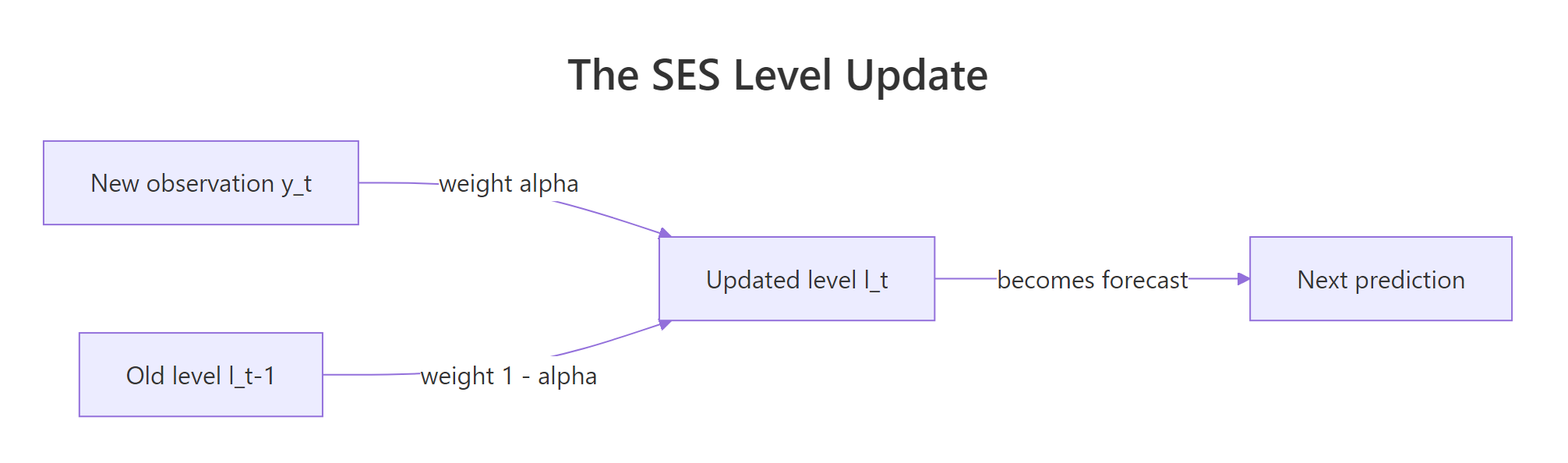
Figure 1: Each new level is a weighted blend of the newest observation and the previous level.
In symbols, writing the level at time $t$ as $\ell_t$:
$$\ell_t = \alpha\, y_t + (1 - \alpha)\,\ell_{t-1}$$
The forecast for any future step is simply the latest level:
$$\hat{y}_{t+h\,|\,t} = \ell_t$$
Alpha lives between 0 and 1, and it decides how much attention each update pays to the newest data point versus everything that came before. The clearest way to feel this is to run the update rule by hand on a tiny series. Below we smooth five numbers with a small alpha of 0.2, starting the level off at the first observation.
Walk through the second step to see the blend. The new observation is 12 and the old level is 10, so the update is 0.2 * 12 + 0.8 * 10 = 10.4. With alpha only 0.2, the level barely moves toward the new 12; it stays close to the old level. That is a slow, heavily smoothed series that barely responds to single-point noise.
Now watch what a large alpha of 0.8 does to the very same numbers.
With alpha 0.8, the second step is 0.8 * 12 + 0.2 * 10 = 11.6, jumping most of the way to the new value. The whole series now chases the data closely, tracking every bump. Compare the two results: alpha 0.2 ends near 10.8 while alpha 0.8 ends near 12.5, much closer to the final observation of 13. Same data and the same update rule produce very different behaviour, all set by one number.
Try it: Smooth the same y vector with alpha = 0.5 and see where the level lands between the slow and fast versions.
Click to reveal solution
Explanation: With alpha 0.5 each update is a straight halfway split between the new observation and the old level, so the result sits neatly between the alpha 0.2 and alpha 0.8 outcomes.
Why do older observations get less weight?
Unrolling the update rule reveals a useful fact: the forecast turns out to be a weighted average of every past observation, where the weights shrink geometrically as you go back in time. Expanding the equation gives:
$$\hat{y}_{T+1\,|\,T} = \alpha y_T + \alpha(1-\alpha) y_{T-1} + \alpha(1-\alpha)^2 y_{T-2} + \cdots$$
The most recent value gets weight $\alpha$, the one before it gets $\alpha(1-\alpha)$, the one before that $\alpha(1-\alpha)^2$, and so on. Each step further back multiplies the weight by another factor of $(1-\alpha)$, so the influence of old data fades away smoothly. That geometric fade is the "exponential" in exponential smoothing. Let's compute those weights directly for alpha 0.2.
The newest observation gets 0.2, the next 0.16, then 0.128, each about 80% of the one before. The weights trail off gently, so observations from many steps back still contribute a little. Because they form a geometric series, all the weights (out to infinity) sum to exactly 1, which is what makes the forecast a proper weighted average.
A larger alpha changes the character of that decay completely. Here are the weights for alpha 0.8.
Now the newest point alone carries 80% of the weight, and by the third step back the weight is already down near zero. A high alpha has a short memory: it essentially forecasts from the last observation or two. A low alpha has a long memory, spreading its attention over many past values. Alpha is really a memory-length dial.
Try it: Compute the weights for alpha = 0.5 and confirm each weight is exactly half the previous one.
Click to reveal solution
Explanation: With alpha 0.5 the decay factor is 1 - 0.5 = 0.5, so every weight is half of the one before it. The series halves at each step: 0.5, 0.25, 0.125, and so on.
How does ses() choose the best alpha automatically?
You do not have to guess alpha. By default, ses() finds the value that makes the model fit the historical data as closely as possible. It measures fit with the sum of squared errors (SSE), the total of the squared gaps between each actual value and the model's one-step-ahead forecast of it:
$$\text{SSE} = \sum_{t=1}^{T} \left(y_t - \hat{y}_{t\,|\,t-1}\right)^2$$
The function searches for the alpha (and the starting level) that make SSE as small as possible. There is no tidy formula for the answer, so R uses numerical optimisation under the hood. You can read the chosen values straight off the fitted model.
The fit reports alpha = 0.2457, a fairly low value, which tells us the Nile level moves gently and rewards a long memory. It also estimates the initial level l = 1110.7341 (the starting point of the recursion, which ses() optimises rather than fixing at the first observation) and sigma, the standard deviation of the residuals (the one-step-ahead forecast errors, the same gaps the SSE above squares and sums). The AIC, AICc, and BIC are model-comparison scores you can use to pit SES against other models.
To prove that alpha 0.2457 really is the SSE minimiser, we can rebuild the search by hand. The loop below tries a grid of alpha values, refits SES at each one, and records the SSE.
The grid minimum lands at 0.25, right next to the 0.2457 that ses() reported. Our search steps in coarse jumps of 0.01, while ses() optimises alpha as a continuous number, which is why the two differ only in the third decimal. A quick plot of the SSE curve shows a clear valley at that alpha.
Try it: Run the same grid search on the built-in LakeHuron series (annual lake level) and see which alpha it prefers.
Click to reveal solution
Explanation: LakeHuron is very persistent from one year to the next, so the best SES leans almost entirely on the most recent value. An alpha near 1 is a hint that SES is barely smoothing at all, a point we return to in the section on when to use SES.
How do you read the forecast and its prediction intervals?
A forecast object carries two things worth reading: how well the model fit the past, and how uncertain it is about the future. The accuracy() function summarises the in-sample fit with a row of error metrics.
The two you will use most are RMSE (root mean squared error, 142.78 here) and MAPE (mean absolute percentage error, 12.95, meaning the fitted values are off by about 13% on average). MASE below 1 means SES beats a naive one-step benchmark on the training data. These numbers describe fit, not future accuracy, but they are a useful first read.
Now the uncertainty. The point forecast is flat, but the prediction intervals are not. The block below forecasts ten years ahead and pulls out the upper 95% bound at each step.
The upper bound climbs from 1088 at one year out to 1156 at ten years out. The point forecast never moves, but the model grows less certain the further ahead it looks, so the band around that flat line keeps widening. That widening is appropriate: SES estimates today's level, but it cannot rule out that the level will drift over the next decade.
Try it: Measure how much the 80% interval widens between the first and tenth forecast step.
Click to reveal solution
Explanation: The 80% band is about 370 units wide one year out and about 459 units wide ten years out. Uncertainty compounds with the horizon even though the point forecast stays put.
When should you use SES (and when not)?
Simple exponential smoothing assumes the series has no trend and no seasonality. If either is present, SES is the wrong tool and its flat forecast will lag reality. The decision is short: check for a trend, then check for a season.
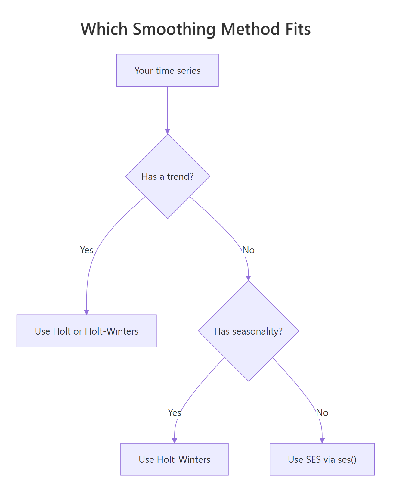
Figure 2: SES fits only when the series has no trend and no seasonality.
When there is a trend, Holt's method adds a slope term; when there is a season too, Holt-Winters adds a seasonal term. SES is the base case, the model for a level that only wanders. To see it fail on purpose, apply SES to an obviously rising series and watch the forecast flatten out.
The data climbs steadily, but the SES forecast is a horizontal line at the last level, missing the trend entirely. That is the picture of a misapplied model.
On a genuine level series, though, SES earns its keep. Here we split the Nile data into a training period and a test period, then compare SES against two simple benchmarks: the naive forecast (carry the last value forward) and the mean forecast (predict the historical average). We score each by RMSE on the held-out test years.
SES wins with the lowest test RMSE (124.33), beating both the naive last-value forecast and the long-run mean. That is exactly the promise from the first section made concrete: SES sits between the two crude baselines and, on a level series, outperforms them both.
Try it: Fit SES to the LakeHuron series, read the estimated alpha, and decide whether SES is really smoothing the data.
Click to reveal solution
Explanation: Alpha is almost exactly 1, so SES is doing essentially no smoothing, it is just repeating the last value like a naive forecast. That is a sign LakeHuron carries year-to-year structure a richer model (such as an AR model or ETS) could exploit.
Complete Example: forecasting New Haven temperature
Let's put every piece together on a fresh dataset. The built-in nhtemp series records the mean annual temperature in New Haven, Connecticut, from 1912 to 1971 in degrees Fahrenheit. It has no seasonal cycle (each value is already a yearly average) and only a faint drift, which makes it a natural fit for SES. We fit the model and read its parameters first.
The optimiser settles on alpha = 0.182, a moderate value that says recent years matter more than distant ones but no single year dominates. Now we check the fit and read the forecast.
The MAPE of 1.749 says the fitted temperatures are within about 1.7% of the actual values, an excellent fit for this smooth series. The forecast holds flat at 51.87 degrees, with a 95% interval of roughly 49.6 to 54.1 in the first year that widens slightly each year after. A quick plot rounds off the workflow.
That is the full loop: fit, inspect alpha, check accuracy, read the forecast and its intervals, and plot the result.
Practice Exercises
These capstone problems combine the ideas above. Each uses fresh variable names so nothing you ran earlier gets overwritten. Try them before opening the solutions.
Exercise 1: Forecast the discoveries series
The built-in discoveries series counts great scientific discoveries per year from 1860 to 1959. Fit SES with a 4-year horizon, report the alpha that ses() chooses, and read off the point forecast.
Click to reveal solution
Explanation: The optimiser picks alpha 0.1756, a low value, so the forecast leans on many past years. As always the point forecast is flat, here about 1.142 discoveries per year.
Exercise 2: Rebuild the final level by hand
Show that the SES forecast really is the last level from the recursion. Fit SES to nhtemp, pull out the estimated alpha and initial level, run the update rule yourself over the whole series, and confirm your final level equals the point forecast.
Click to reveal solution
Explanation: Starting from the optimised initial level l and applying the update rule with the optimised alpha reproduces the forecast exactly (51.8705). The point forecast is nothing more than the final smoothed level.
Exercise 3: Does SES beat a naive forecast on the Nile?
Split the Nile series into a training set (up to 1955) and a test set (1956 onward). Fit SES and a naive forecast on the training set, then compare their RMSE on the test set. Which one would you trust?
Click to reveal solution
Explanation: SES posts a lower test RMSE (124.33) than the naive forecast (129.21), so on this level series the smoothed forecast generalises better than simply repeating the last value.
Frequently Asked Questions
What is the difference between SES and a moving average?
A moving average gives every observation in its window the same weight and ignores everything outside the window. Simple exponential smoothing keeps all of history but weights it, so recent values matter more and old values fade smoothly. That gentle fade is why SES usually reacts to change faster than a moving average of comparable smoothness.
What alpha value should I choose?
In almost every case, let ses() choose it for you by minimising the sum of squared errors. If you must set it by hand, low values (0.1 to 0.3) suit noisy series where you want a stable, smooth forecast, and higher values suit series where recent observations really do carry the most information. An estimated alpha near 1 is a signal that SES may be too simple for the data.
Can SES forecast data with a trend or seasonality?
No. Simple exponential smoothing models a level only, so it will flatten any trend and ignore any season. For a trending series use Holt's method, and for a seasonal series use Holt-Winters or let ets() pick the right components automatically.
Why is the SES forecast a flat line?
Because SES tracks a single quantity, the current level, and its forecast for every future step is that same level. With no trend term to add a slope and no seasonal term to add a cycle, the point forecast has nowhere to go, so it stays flat while only the prediction intervals widen.
How is ses() related to HoltWinters() and ets()?
All three fit exponential smoothing models. Base R's HoltWinters() can do simple smoothing too but minimises one-step errors slightly differently and lacks the tidy forecast object. The forecast package's ses() is a friendly wrapper around ets() restricted to the level-only model (known as ETS(A,N,N), meaning additive error, no trend, no season). Use ses() for clarity when you specifically want simple exponential smoothing, and ets() when you want the software to compare model forms for you.
Summary
Simple exponential smoothing is the base model of the exponential smoothing family: one level, one parameter, a flat forecast. Everything flows from the alpha smoothing parameter.
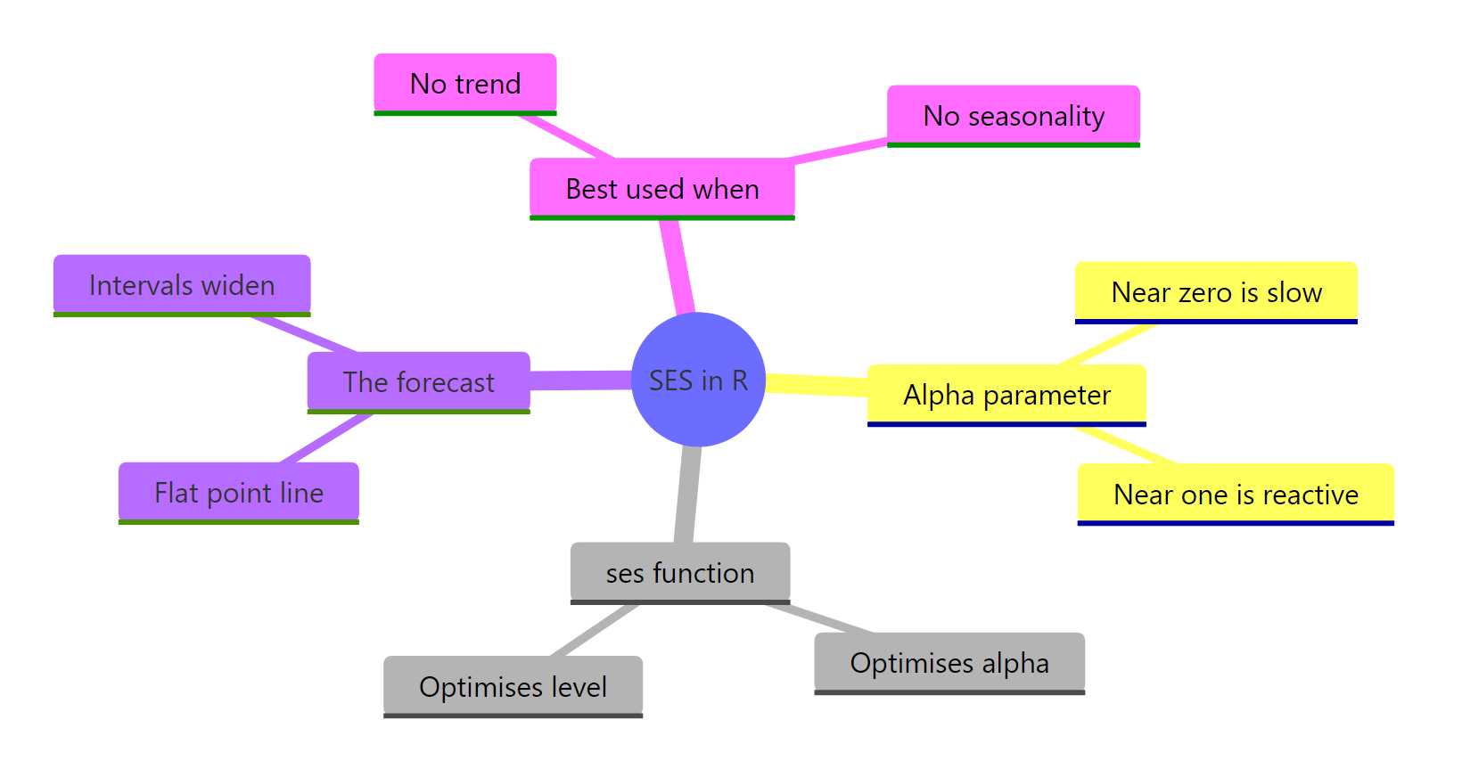
Figure 3: The moving parts of simple exponential smoothing in R.
| Idea | What to remember |
|---|---|
| The model | Each level is alpha * new value + (1 - alpha) * old level; the forecast is the latest level |
| Alpha | Between 0 and 1; near 0 means slow and smooth (long memory), near 1 means reactive (short memory) |
| Weights | Past observations get geometrically decaying weight alpha * (1 - alpha)^j, summing to 1 |
| ses() | Picks alpha and the initial level by minimising the sum of squared errors |
| The forecast | A flat point forecast with prediction intervals that widen over the horizon |
| When to use it | Only for series with no trend and no seasonality; an alpha near 1 hints the method is too simple |
The ses() function packages all of this into one call: it fits the level, optimises alpha, and returns a forecast with prediction intervals that widen with the horizon. Reach for it whenever you have a series that drifts around a level without marching up or cycling through seasons.
References
- Hyndman, R.J. & Athanasopoulos, G. Forecasting: Principles and Practice, 2nd edition, Section 7.1: Simple exponential smoothing. Link
- Hyndman, R.J. & Athanasopoulos, G. Forecasting: Principles and Practice, 3rd edition, Section 8.1: Simple exponential smoothing. Link
- Hyndman, R.J. et al. forecast package documentation,
ses()andets()reference. Link - forecast package on CRAN. Link
- NIST/SEMATECH e-Handbook of Statistical Methods, Section 6.4.3.1: Single Exponential Smoothing. Link
- R Core Team.
Nileandnhtempdatasets, R datasets package documentation. Link
Continue Learning
- ETS Models in R: the
ets()function generalises SES, adding trend and seasonality and picking the best model form automatically. - Holt-Winters in R: extend smoothing to series that have both a trend and a repeating seasonal cycle.
- Moving Averages in R: the equal-weight cousin of exponential smoothing, and a good contrast for understanding why weighting recent data helps.