Combining Forecasts in R: Ensemble Averaging
Combining forecasts means averaging the predictions of several models into a single number instead of picking one model and trusting it. It usually beats the average model you could have picked, because the models make mistakes in different directions and those mistakes partly cancel when you add them up.
What does combining forecasts actually mean?
Picking a forecasting model is a bet. Fit exponential smoothing and ARIMA to the same series and they will hand you different numbers for next month, and there is no reliable way to know in advance which one to trust. Combining sidesteps the bet entirely: you keep both, and you average them. Let's watch that happen on a series you have almost certainly seen before.
We will use AirPassengers, which ships with R. It records the monthly total of international airline passengers, in thousands, from January 1949 to December 1960. It trends upward and it has a strong yearly cycle, which makes it a fair test for any forecasting method.
The rule we have to follow is simple: hide some of the data, forecast it, then check. We will train on everything up to the end of 1959 and hold back the twelve months of 1960 as the answer sheet.
window() cuts a slice out of a time series using calendar positions rather than row numbers, so end = c(1959, 12) means "up to and including December 1959". We now have 132 months to learn from and 12 months that the models are not allowed to see.
Next we fit three genuinely different forecasting methods and ask each for the twelve months of 1960. You do not need to understand their internals to follow this article. All that matters is that they work in different ways, so they make different mistakes.
ets()fits an exponential smoothing model, which builds a forecast from weighted averages of recent values.auto.arima()searches a family of ARIMA models, which forecast from past values and past errors.stlf()first splits the series into trend, season and remainder, forecasts the deseasonalised part, then puts the season back.
Each forecast() call returns an object whose $mean component holds the predicted values, one per future month. cbind() glues those three columns next to the truth so we can read across a row and see all four numbers for the same month.
Read the July 1960 row. The truth was 622. ETS said 569.9, ARIMA said 612.9, STL said 544.9. The three models disagree by nearly 70 passengers about the same month, and every one of them undershoots. Now look at November: ETS says 376.6 and ARIMA says 426.9, and this time the truth (390) sits near the bottom rather than the top. The models are not simply ranked best to worst. They take turns being wrong.
That is the opening for combining. If we just average the three columns, the months where one model runs high and another runs low should partly settle down.
The combination is one line of arithmetic: add the three $mean vectors and divide by three. The rmse() helper is the root mean squared error, the usual way to score a forecast. It squares each miss, averages the squares, and takes the square root, so it is measured in passengers and bigger misses count for more. Lower is better. The row labelled STL-ETS is the stlf() forecast, named that way because stlf() uses exponential smoothing on the deseasonalised series; later tables shorten the label to STL.
The combination scored 22.26, which is lower than all three of the models it was built from. The best single model, ARIMA, scored 23.93. So this average of three forecasts, none of which required any tuning or judgement, beat every one of its own ingredients.
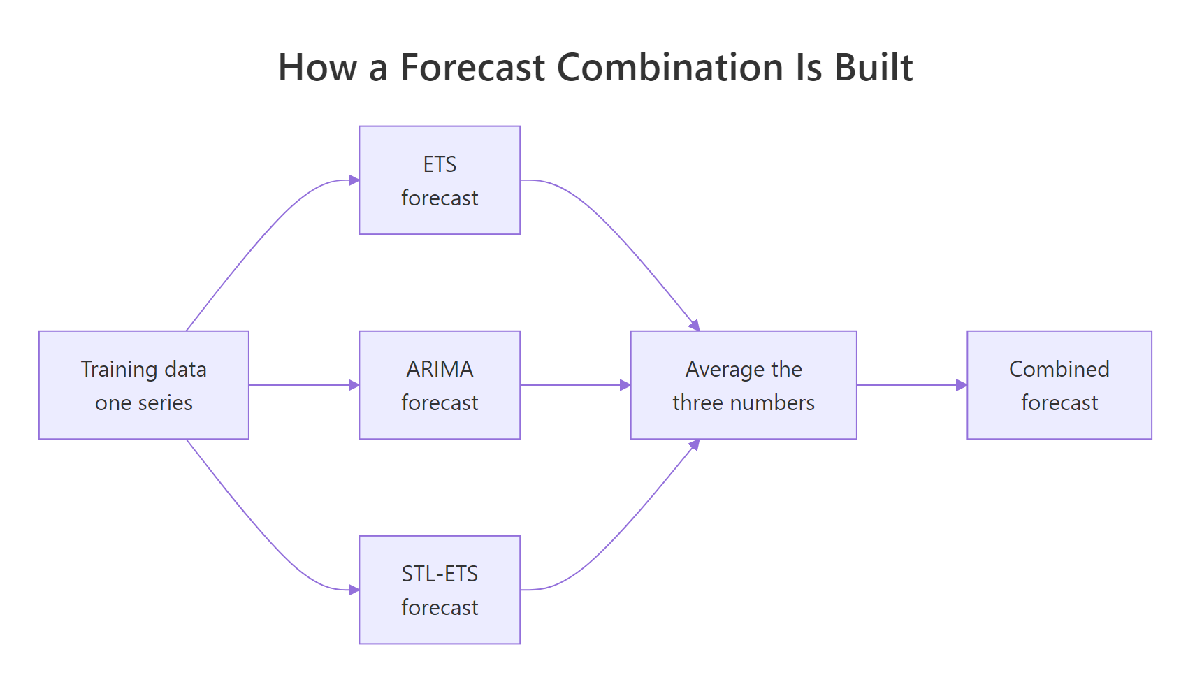
Figure 1: One training series feeds three models, and their three forecasts collapse into one number.
Try it: RMSE punishes large misses harshly because it squares them. Check whether the combination still wins under mean absolute error, which just averages the size of each miss without squaring.
Click to reveal solution
Explanation: The ranking is unchanged and the combination still wins, at 17.61 against ARIMA's 18.53. That matters, because a result that only appears under one error measure is usually an artefact of that measure. This one is not.
Why does averaging forecasts beat the models it averages?
The last section showed that combining worked. It did not show why, and "the errors cancel" is a slogan until you can point at the numbers. So let's point at them. We will subtract each model's forecast from the truth and look at the twelve misses, month by month.
A positive number means the model forecast too low and the truth came in above it. A negative number means the model overshot. Because test and each $mean are both monthly time series covering 1960, R lines them up by date automatically before subtracting.
Now read December. ETS was 7.2 too low while ARIMA was 37.9 too high. Average those two and you get a miss of about 15 instead of 38. That is the cancellation, and it is happening for real in the table, not in a diagram. August is the same story with the signs flipped between ETS and ARIMA.
March is the opposite case and it is just as important. Every model undershot by a lot: -48.3, -51.8, -29.2. There is nothing to cancel, so the average is still badly wrong. Combining rescues you from disagreement, never from a mistake all your models share.
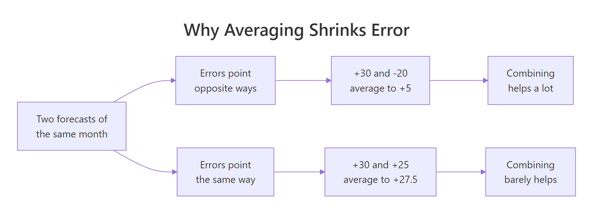
Figure 2: Averaging only helps when the models are wrong in different directions.
We can measure how much the models tend to agree by correlating their error columns. A correlation near 1 means two models miss together, which leaves nothing to cancel. A correlation near 0 means they miss independently.
ETS and STL correlate at 0.878, the highest pair in the table, and that makes sense once you know that stlf() uses exponential smoothing internally on the deseasonalised series. They share most of their machinery, so they tend to miss in the same direction. ETS and ARIMA correlate at 0.676, the lowest pair, because they are genuinely different machinery. That pair is where most of the cancellation comes from.
The identity that makes this a guarantee
So far this is an observation about one dataset. It is actually a mathematical certainty, and the proof is short enough to state. Skip to the code block below if you would rather see it than read it.
Write $e_i$ for the error of model $i$ on some month and $\bar{e}$ for the error of the equal-weight combination. Since the combination is the average of the forecasts, its error is the average of the errors: $\bar{e} = \frac{1}{M}\sum_{i=1}^{M} e_i$. Squaring and averaging over the $M$ models gives an exact split:
$$\text{MSE}_{\text{combo}} = \frac{1}{M}\sum_{i=1}^{M}\text{MSE}_i \;-\; \overline{\text{disagreement}}$$
Where:
- $M$ = the number of models being combined, which is 3 here
- $\text{MSE}_{\text{combo}}$ = the mean squared error of the combined forecast
- $\text{MSE}_i$ = the mean squared error of model $i$ on its own
- $\overline{\text{disagreement}}$ = the average spread of the models' forecasts around their own mean, computed month by month
This is the ambiguity decomposition, known from ensemble learning [4]. Read the right hand side again: you start from the average member's error and you subtract something that can never be negative, because a spread is a squared quantity. So the combination is never worse than the average member. Not usually, not on average. Never.
Rather than take that on faith, let's compute both sides and check that they match.
The apply(members, 1, ...) line walks through the twelve months one at a time. For each month it takes the three forecasts, measures how far each sits from their own average, squares those distances and averages them. That single number is how much the models disagreed about that month, and disagreement is its average across the year.
The last two numbers are identical: 495.33 and 495.33. The identity is not an approximation. The models' average error was 830.90, their disagreement was worth 335.57, and the combination collected every bit of that difference.
Try it: ETS and ARIMA had the least correlated errors, so their pair should show a large disagreement term. Run the decomposition on just those two and predict their combination's RMSE without ever averaging the forecasts.
Click to reveal solution
Explanation: The pair scores 19.19, better than the three-model combination's 22.26. Dropping STL helped, because STL was both the weakest member and the one most correlated with ETS. Keep that result in mind and stay sceptical of it: you only know STL was the weak link because you have already seen 1960. Section five asks whether you could have known it beforehand.
Did the combination just get lucky on this one test window?
One good year proves very little. The 1960 result could be a coincidence of that particular twelve months, and any honest test has to repeat the exercise on windows we have not already looked at.
So we will roll the origin backwards. Train on everything up to the end of 1955 and forecast 1956, then train up to the end of 1956 and forecast 1957, and so on through 1960. Five separate forecasting problems, five separate scorecards, and the models get refitted from scratch every time.
one_year() packages the whole experiment for a single origin: cut the training window, cut the matching test year, refit all three models, then average them and return five numbers. sapply() runs it once per origin and t() turns the result into one row per year. This block refits three models five times, so give it a few seconds.
The refitting matters. If we reused the models fitted on data through 1959 to forecast 1956, they would have seen the future, and the whole test would be meaningless.
Now the summary that actually answers the question. For each year, did the combination beat the average of the three models, and did it beat whichever model happened to be best that year?
Look at the beat_average column: five TRUEs out of five. That is the guarantee from the previous section showing up in data, exactly as the algebra promised. It could not have come out any other way.
Now look at beat_best: only two TRUEs against three FALSEs. In 1956 and 1957 the combination lost badly to ARIMA on its own, 16.9 against 10.4 and 24.5 against 15.8. Averaging in two weaker models diluted a genuinely strong one.
Averaged over the five years, ARIMA scored 23.84 and the combination scored 26.45. On this series, the honest verdict is that ARIMA was consistently the strongest model and combining it with the others made things slightly worse.
That result is the honest one, and it is the point of the section. Combining is insurance rather than a route to first place. It reliably keeps you out of the bottom half of your model set, which is worth a lot when you cannot tell in advance which model is strong. What it will not do is beat a model that was better all along, and pretending otherwise would leave you unable to explain a year like 1956.
Try it: The guarantee protects you from being average. Check the stronger everyday claim: how often did the combination beat the worst model of the three?
Click to reveal solution
Explanation: Five out of five, which also follows from the guarantee: if the combination always beats the average member, and the average is always below the worst, then the combination always beats the worst. You cannot pick the ruinous model by accident if you refuse to pick at all.
What happens when one of the forecasts is bad?
Everything so far assumed three reasonable models. Real ensembles are messier. Somebody adds a model that made sense last quarter, or a colleague's spreadsheet gets included, or a method quietly breaks when the season shifts. What does one bad member do to the average?
Let's find out by deliberately adding two weak forecasters. A seasonal naive forecast just repeats last year's value for the same month, ignoring the trend entirely. A drift forecast draws a straight line through the first and last training points, ignoring the season entirely. Both are legitimate baselines, and both are badly suited to a series that trends and cycles at the same time.
The two newcomers are far worse than anything we had. Seasonal naive is at 50.71, roughly double the good models. Drift is at 92.67, nearly four times ARIMA, because a straight line simply cannot reproduce a summer peak.
Now we combine all five, three ways. The plain mean weights every member equally, including the bad ones. The median takes the middle value of the five and ignores the rest. The trimmed mean throws away the highest and lowest forecast for each month and averages what survives.
apply(five, 1, median) runs across each month's five forecasts and keeps the middle one. trim = 0.2 tells mean() to discard the top 20% and bottom 20% of the values before averaging, which with five members means dropping one from each end and averaging the middle three.
The plain mean collapsed from 22.26 to 37.35. Two bad members out of five were enough to make the combination worse than any of the three good models individually. The median and the trimmed mean both recover about half of that loss, landing near 32.5, because a single extreme forecast cannot move a middle value the way it moves an average.
Half the damage is still damage. Look at what the bad members do to the actual numbers.
In April the truth was 461. The drift forecast said 413.9, so far below the others that it pulled the mean down to 432.4 while the median stayed at 440.5. Drift makes the same kind of error every month, because a straight line cannot climb for the summer peak, so it pulls the mean down in every row of the table.
Try it: Suppose only the seasonal naive model sneaks in, and the truly awful drift model does not. Combine the three good models plus seasonal naive, and compare the mean against the median. Guess which wins before you run it.
Click to reveal solution
Explanation: The mean wins this time, 25.08 against 28.89, reversing the result from the five-member case. Seasonal naive is mediocre but not extreme, so the mean absorbs it without much harm while the median pays a real price for discarding two of the three good forecasts. Robustness is not free, and it only pays for itself when a member is genuinely far out.
Should you weight the forecasts by how accurate they have been?
Equal weights feel crude. ARIMA has looked stronger than STL all article, so surely we should give it more say. This is the most natural improvement anyone thinks of, it has a long research literature behind it, and it usually does not work. Let's see why.
The classic scheme, from Bates and Granger's original 1969 paper [2], gives each model a weight proportional to the inverse of its squared error, so accurate models get more say:
$$w_i = \frac{1 / \text{MSE}_i}{\sum_{j=1}^{M} 1 / \text{MSE}_j}$$
Where:
- $w_i$ = the weight given to model $i$, and the weights sum to 1
- $\text{MSE}_i$ = the mean squared error of model $i$, measured on data the weights are allowed to see
That last clause is doing the heavy lifting. The weights must come from data that is not the test set, otherwise we are grading our own homework. The safe source is each model's fit on the training data.
accuracy() on a forecast object returns a small table of error measures, and the "Training set" row is how well the model reproduced the data it was fitted to. Notice the numbers are nearly identical: 9.35, 9.91, 9.86. All three models describe the past about equally well.
Notice also that ETS looks best in-sample at 9.35, even though ARIMA was clearly best on the future. Hold that thought.
The weights land at 0.358, 0.319 and 0.322. Equal weights would be 0.333 each. Because the training errors were so similar, the scheme barely moves away from a plain average, and the tiny nudge it does make favours ETS, which was not the model that deserved it.
Equal weights 22.26, inverse-MSE weights 22.39. The sophisticated scheme is very slightly worse. This is the forecast combination puzzle: theoretically better weighting schemes keep failing to beat the simple average in practice [5].
What happens if we estimate the weights properly
Maybe inverse-MSE is too timid. Granger and Ramanathan proposed treating the whole thing as a regression: put the actual values on the left, the member forecasts on the right, and let least squares find the weights. That is strictly more flexible, so it should do strictly better.
To keep it honest we need a third slice of data. We will train the models on everything through 1958, forecast 1959, then fit the regression on that year. Then we apply those weights to the 1960 forecasts we already have.
lm() fits a linear regression: the variable on the left of ~ is predicted from the variables on the right, and coef() pulls out the fitted intercept and slopes. Look at what the regression decided. ETS gets a weight of -0.893, meaning "whatever ETS says, move away from it". STL gets 2.624, more than double its own forecast. And there is an intercept of -214.5 on top. These are not weights in any meaningful sense. Least squares had four free parameters and only twelve months to fit, so it picked whatever coefficients minimised the error on those twelve months, however implausible they look.
The regression weights scored 68.32, three times worse than simply averaging. The most flexible method available produced the worst forecast in this article by a wide margin, because it spent all its flexibility memorising the noise in a single validation year.
For completeness, here is the ceiling nobody can reach. Fit the same regression directly on the 1960 test data, which is cheating, and see how good the weights could theoretically have been.
The residuals of that fit are exactly the errors the oracle combination would have made, so the square root of their mean square is its RMSE. Perfect hindsight weights would have scored 12.31 against the simple average's 22.26. So there really is a much better combination in there. The problem is that finding it requires knowing the answer, and every honest attempt to estimate it from real data made things worse instead.
Try it: ARIMA was the strongest model on the test year. Try tilting the combination toward it by hand: 0.5 to ARIMA, 0.3 to ETS, 0.2 to STL. Remember this uses hindsight you would not have had.
Click to reveal solution
Explanation: 19.85 beats the equal-weight 22.26, and it also beats every automatic weighting scheme we tried. That is not a recommendation. You chose those weights by reading the test-set scoreboard, which is the one thing you can never do with a real forecast. It does show that good weights exist, which is why researchers keep looking for a way to estimate them.
How do you build a prediction interval for a combined forecast?
A point forecast is half an answer. Anyone acting on it needs a range too. Each of our three models supplies its own 95% interval, so the tempting move is to average the lower bounds and average the upper bounds. That is wrong, and it is worth seeing why.
The $lower and $upper components of a forecast object are matrices with one column per confidence level. Column 1 holds the 80% bounds and column 2 the 95% bounds, so [, 2] picks the 95% interval.
The March row exposes the problem. The truth was 419 and the interval runs from 423.7 to 500.6, so the actual value falls outside a 95% interval entirely. That can happen once in a while by chance, but the deeper issue is structural: this interval only describes how uncertain each model is about its own forecast. It says nothing about the fact that the three models disagree with each other by 22 passengers about that very month.
The honest way to combine uncertainty is to treat the ensemble as a mixture: with probability one third the world behaves like the ETS model, with probability one third like ARIMA, and with probability one third like STL. We simulate from that mixture and read the quantiles off the pooled draws.
First we need each model's mean and standard deviation at each horizon. The standard deviation is recoverable from the 95% bound, since a 95% upper bound sits 1.96 standard deviations above the mean.
qnorm(0.975) is 1.959964, the number of standard deviations that leaves 2.5% in the upper tail of a normal distribution. Dividing the distance from the mean to the upper bound by it recovers the standard deviation. The spreads widen from January to April, which is the usual pattern: the further ahead you forecast, the less you know.
Now the simulation. For each of the twelve months we draw four thousand futures. Each draw picks one of the three models at random, then draws a value from that model's own distribution for that month.
sample(1:3, n_sim, replace = TRUE) chooses a model for each of the four thousand draws. Because mean_mat[h, pick] is indexed by that vector of choices, rnorm() receives four thousand mean and standard deviation pairs at once and returns one draw from each. set.seed(2026) fixes the random numbers so you get exactly these results.
The result is a 4000 by 12 matrix: four thousand possible versions of 1960. The interval is just the middle 95% of each column.
March now runs from 417.5 to 506.9, and the actual value of 419 sits inside it. The lower bound moved down by six passengers, which is precisely the model disagreement that the averaged-bounds version had thrown away.
Let's measure both versions properly: how wide are they on average, and how often did they actually contain the truth?
The pooled interval is 125.7 passengers wide against the naive version's 107.1, about 17% wider. It captured all twelve actual values while the averaged-bounds interval captured eleven, so 91.7% coverage from something that claimed to be a 95% interval.
Twelve months is far too small a sample to judge coverage properly, so do not read much into 11 versus 12. The structural argument is the one that should convince you: across the twelve months, the gap between the highest and the lowest member forecast averages 38 passengers, and any interval built by averaging the members' own bounds is arithmetically incapable of reflecting that.
Try it: Build an 80% interval instead of a 95% one from the same draws matrix, and check how wide it is.
Click to reveal solution
Explanation: The 80% interval is 83.4 wide, a third narrower than the 95% one, and it still caught eleven of twelve months. Demanding less confidence buys you a tighter range. You have learned nothing new about 1960, you have simply agreed to be wrong more often.
Which R packages combine forecasts for you?
Everything so far was deliberately hand-rolled, because a combination really is just arithmetic on vectors and you should be able to see that. For production work there are packages that handle the bookkeeping, and the modern one is fable, which lets you write a combination as an algebraic expression over fitted models.
|> is R's pipe: it feeds the value on its left into the function on its right as the first argument, so air |> filter(...) means the same as filter(air, ...). as_tsibble() converts the classic time series object into a tsibble, the tidy time series format the fable ecosystem uses. model() fits several models in one call and returns a mable, a table with one column per fitted model. The clever part is the mutate() line: (ets + arima) / 2 is real arithmetic on model objects, and fable stores the result as a first-class model of type COMBINATION.
Because the combination is a model like any other, forecasting and scoring it need no special handling.
Passing air, the full series, to fabletools::accuracy() is what lets it look up the true 1960 values and score each forecast against them. The ARIMA that fable selected differs from the one auto.arima() chose, so its score differs too. The pattern is the one we have seen all article: the combination lands between its members, well clear of the weaker one.
library(fable) a bare accuracy() call is the fabletools version and will reject a plain forecast object. Write fabletools::accuracy() or forecast::accuracy() explicitly whenever both are loaded.Here is how the main options compare.
| Package | How you combine | Best for |
|---|---|---|
fable |
Algebra on fitted models, (ets + arima) / 2 |
Modern tidy workflows, actively maintained |
forecast |
Manual arithmetic on $mean vectors |
Full control, and it is what this article used |
forecastHybrid |
hybridModel() fits five methods and weights them |
A quick ensemble with no setup |
opera |
Weights updated online as new data arrives | Long live series where the best model changes over time |
ForecastComb |
Fifteen schemes including eigenvector methods | Research comparisons across many weighting rules |
opera starts earning its place.Try it: Add a seasonal naive model to the fable combination and see what a weak third member does inside the tidy workflow.
Click to reveal solution
Explanation: Adding seasonal naive pushed the combination from 22.3 to 28.3, now worse than ETS alone. The tidy syntax makes bad ensembles just as easy to build as good ones. Nothing in fable will warn you that a member is dragging the average down, so screening remains your job.
Complete Example
Here is the whole workflow wrapped into one reusable function. Give it a seasonal series, a forecast horizon and a combining rule, and it splits the data, fits three models, combines them and scores everything.
USAccDeaths counts monthly accidental deaths in the United States, a series with no strong trend, which makes it a completely different test from AirPassengers. Inside the function, head() and tail() cut the series into its first n - h and last h values, and ts() rebuilds each piece as a time series: start(y) and frequency(y) carry over the original calendar, and time(y)[n - h + 1] is the calendar time of the first test point. switch() picks the combining rule from the string you passed, and as.numeric() inside rmse() strips the time series attributes so the subtraction works whether combined came back as a series or a plain vector.
The result is the pattern this article has been building toward, in miniature. The combination scored 278.75, below the members' average of 283.4, above the best member's 271.88. It beat two of three models without knowing in advance which two.
One function, any series. Let's point it at a quarterly one.
UKgas is quarterly UK gas consumption, so we hold out eight quarters instead of twelve months and the function adapts automatically through frequency(y). Once again the combination at 84.05 beats the members' average of 86.35 and lands between the best and the worst member. That is the same outcome we got on AirPassengers and on USAccDeaths, on three series with quite different shapes.
Practice Exercises
Exercise 1: Verify the guarantee on a different year
The ambiguity decomposition should hold for any holdout window, not just 1960. Refit all three models on data through 1958, forecast the twelve months of 1959, and confirm that average member MSE - disagreement equals the combination's actual MSE. Report the combination's RMSE both ways.
Click to reveal solution
Explanation: The two RMSE figures agree to the decimal, 48.44 and 48.44, so the identity holds on 1959 exactly as it did on 1960. Note how small the disagreement term is here, 99.91 against 1960's 335.57. The models largely agreed about 1959 and were largely wrong together, which is why the combination saved so little that year.
Exercise 2: Screen out the weakest member, honestly
The try-it in section two showed that the ETS and ARIMA pair beat the three-model combination on 1960. Try to reach that result without cheating: use each model's training RMSE to identify the weakest member, then drop it and average the two survivors. Compare against the mean of all three.
Click to reveal solution
Explanation: Honest screening dropped ARIMA, which was the best model on the future and only looked worst on the past. The screened pair scored 30.05 against the unscreened 22.26, so the attempt to be clever raised the error by 35%. In-sample fit is a poor guide to out-of-sample skill, and that is the same force that makes estimated weights fail. Screening is for members you know are broken, not for members that fit the training data marginally less tightly.
Exercise 3: Robust rules on a different series
Build a five-member ensemble on USAccDeaths, holding out 1978. Use ETS, ARIMA, STL, seasonal naive and drift, then compare the mean, median and trimmed mean. Decide which rule you would ship.
Click to reveal solution
Explanation: The median wins clearly at 277.03, cutting 23% off the plain mean's 361.39, with the trimmed mean close behind at 290.51. This reproduces the section four result on a completely different series, which is the kind of repetition that should raise your confidence in a finding. Ship the median whenever you have five or more members and cannot vouch for all of them.
Frequently asked questions
How many forecasts should I combine?
Three to five is the sweet spot for most work. Two models give you one cancellation opportunity per period, which is thin. Beyond about five, each extra member changes the average less and less, so the effort goes into finding a genuinely different method rather than adding a fourth variation on exponential smoothing. If you do go past five, switch from the mean to the median, because a large ensemble is much more likely to contain a broken member.
Can I combine forecasts from models fitted on transformed data?
Yes, as long as you transform everything back to the original scale before averaging. If one model forecasts log passengers and another forecasts passengers, averaging them directly is meaningless. Exponentiate the log forecast first. Be aware that the exponential of a mean is not the mean of the exponentials, so back-transformed forecasts carry a small bias; forecast() handles this for you when you pass lambda and biasadj = TRUE.
Should I combine a machine learning model with a statistical one?
That is often the best pairing you can build, precisely because the two make errors for different reasons. A gradient boosting model and an ARIMA will rarely be wrong in the same direction on the same month. The only requirement is that both produce forecasts for the same periods on the same scale. Everything in this article applies unchanged, since the combination never looks inside its members.
My combination is worse than my single best model. What should I do?
First check whether you know it is your best model, or whether you only know it was best on the window you just measured. Exercise 2 above showed a model that looked worst on the training data and turned out best on the future. If you have several years of rolling evidence that one method consistently wins, then trusting it is reasonable. If you have one holdout window, you are probably looking at noise, and the combination is the safer choice.
Do I have to refit all the models every time new data arrives?
Refit on the same schedule you would use for a single model. The combination adds no new fitting requirement, it just multiplies the work by the number of members. If refitting is expensive, note that the weights in an equal-weight combination never need re-estimating, which is one more practical advantage of the simple average over anything data-driven.
Does this work for weekly or daily data?
The arithmetic is identical at any frequency. What changes is which members are worth including, since methods like ets() struggle with the long seasonal periods that daily and weekly data bring. For high-frequency series, build your ensemble from methods designed for it, such as tbats(), dynamic harmonic regression, or Prophet, then average them exactly as we did here.
Summary
Combining forecasts is one of the few techniques in forecasting that is simultaneously trivial to implement and hard to beat. The arithmetic is a single division. Everything difficult about it is knowing what it does and does not promise.
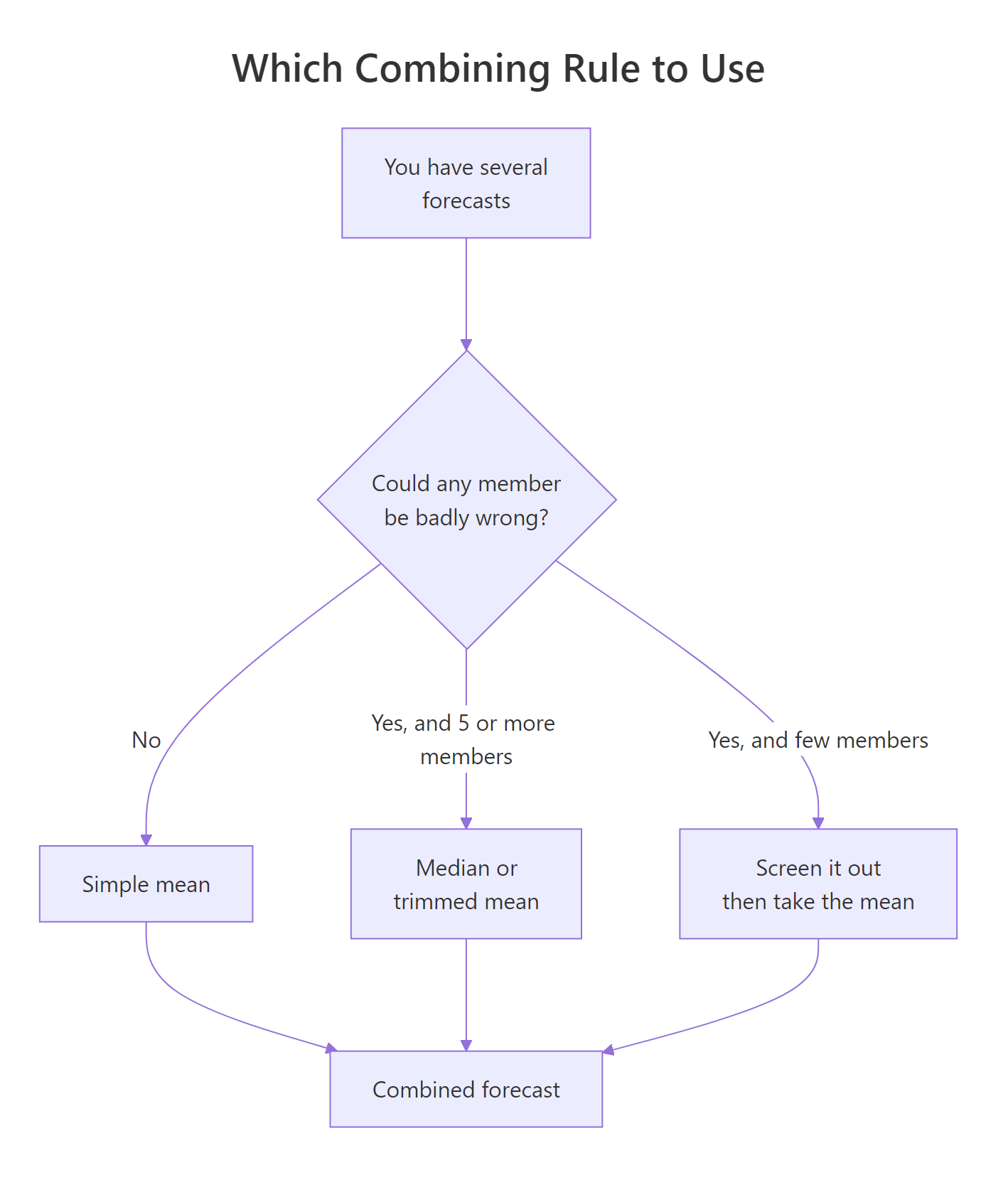
Figure 3: Choosing between the mean, the median and screening.
| What you learned | The takeaway |
|---|---|
| How to combine | Average the $mean vectors of several forecast objects, then score as usual |
| Why it works | Errors of different sign cancel, and the ambiguity decomposition makes the gain exact |
| What is guaranteed | The combination can never be worse than the average member, on any data |
| What is not guaranteed | It may lose to the single best member, and on AirPassengers it lost to ARIMA 3 years in 5 |
| Which members to pick | Diversity beats individual accuracy, since correlated models leave nothing to cancel |
| When one member is bad | The equal-weight mean is poisoned; use the median with 5 or more members, or screen first |
| Whether to weight | Inverse-MSE barely moved the needle, and regression weights scored 3 times worse than a simple average |
| How to build intervals | Pool simulated futures across models; averaging the members' bounds understates uncertainty |
| Which package | fable for tidy workflows, plain forecast arithmetic for full control |
The single most useful habit from all of this is to stop treating model selection as a decision you must get right. If you have three plausible models and no strong reason to prefer one, average them and move on to a problem where your judgement actually adds value.
References
- Hyndman, R.J. & Athanasopoulos, G. Forecasting: Principles and Practice, 3rd edition, Section 13.4: Forecast combinations. Link
- Bates, J.M. & Granger, C.W.J. The Combination of Forecasts. Operational Research Quarterly 20(4), 451-468 (1969). The paper that started the field; it sits behind a paywall, and reference 3 summarises its argument.
- Wang, X., Hyndman, R.J., Li, F. & Kang, Y. Forecast combinations: an over 50-year review. International Journal of Forecasting (2023). Link
- Krogh, A. & Vedelsby, J. Neural Network Ensembles, Cross Validation, and Active Learning. NeurIPS (1994), the origin of the ambiguity decomposition. Link
- Lee, S. & Lee, T.-H. Solving the Forecast Combination Puzzle. University of California Riverside working paper 202514. Link
- Makridakis, S., Spiliotis, E. & Assimakopoulos, V. The M4 Competition, where combinations dominated the leaderboard. Methods and results archive. Link
- Hyndman, R.J. forecast: Forecasting Functions for Time Series and Linear Models, CRAN reference manual. Link
- Hyndman, R.J. R packages for forecast combinations, comparing opera and forecastHybrid. Link
- O'Hara-Wild, M., Hyndman, R.J. & Wang, E. fable: Forecasting Models for Tidy Time Series. Link
- Hyndman, R.J. & Athanasopoulos, G. Forecasting: Principles and Practice, Section 5.10: Time series cross-validation. Link
Continue Learning
- Forecast Accuracy in R covers RMSE, MAE, MAPE and MASE in depth, including which measure to trust when your series changes scale.
- Time Series Cross-Validation in R turns the five-origin test from section three into a proper automated procedure with
tsCV(). - ETS vs ARIMA in R explains what the two main members of our ensemble actually do, and why their errors are so different.
- Prediction Intervals in R goes deeper on interval width, coverage and what breaks when residuals are not normal.