Missing Values in Time Series: Imputation That Keeps the Season
Imputing a time series means filling its gaps with values that preserve how each observation relates to its own past. That relationship, called autocorrelation, is what every forecasting method actually reads. Fill the holes carelessly and you do not just get a few wrong numbers, you hand the next model a series whose memory has been rewritten.
What breaks when you fill a time series with the mean?
The habit is almost automatic. There are NA values in the column, so you reach for mean(x, na.rm = TRUE) and paint it over every hole. In a spreadsheet of customer ages that is defensible. In a time series it quietly destroys the thing you are about to model.
To see the damage we need a series whose true values we already know, so we can compare. R ships with nottem, twenty years of monthly average air temperature at Nottingham Castle, with no missing values at all. We will knock holes in it ourselves: a twelve-month logger outage, plus twenty-four scattered dropouts.
Two numbers tell the story. The standard deviation says how much the series moves. The autocorrelation at lag 12 says how strongly each month resembles the same month a year earlier, which for monthly temperature should be very strong indeed. One detail about reading it off: acf() returns the whole run of autocorrelations starting at lag 0, so the lag-12 value sits in position 13 of $acf.
Fifteen percent of the values are gone and we replaced them with a constant. The standard deviation dropped from 8.57 to 7.77, because a constant contributes no variation. More seriously, the year-over-year autocorrelation fell from 0.884 to 0.729. The series still looks like temperature data, but its seasonal memory has been visibly weakened, and every seasonal model you fit next will inherit that weakening.
Look at what the mean actually put into the outage year to see why.
The real January was 41.6 and the real August was 61.6, a swing of twenty degrees. The mean fill claims both months were 49.02. It has asserted that this particular year had no summer and no winter. Averaged over the whole series that value is perfectly reasonable, which is exactly what makes the error so easy to miss: nothing looks obviously wrong until you check the seasonal structure.
Try it: Autocorrelation at lag 1 measures how much each month resembles the month directly before it. Compute it for temps and for mean_filled and see whether mean filling hurt the short-range memory too.
Click to reveal solution
Explanation: acf() returns lag 0 in position 1, so the lag-1 value sits in position 2. Short-range memory took the same kind of hit as the seasonal memory, falling from 0.808 to 0.692. Every imputed point sits at the series average, so it neither follows the point before it nor leads the point after it.
Where are your gaps, and are they even visible?
Before choosing a repair you need to know exactly what you are repairing. That means three questions in order: are all the gaps visible at all, how long are they, and is there a pattern in where they fall.
Start with visibility, because this is where most real projects go wrong. A time series can be missing data in two completely different ways. Either the row is present and the value is NA, or the row is simply not there. Only the first kind is visible to is.na().
Here are six daily water-level readings from a logger. Count the missing values.
Zero missing values, says R. Now read the dates. The 3rd, 4th, 7th and 8th of March never appear. Four days of data are gone, and the standard check reports a clean dataset, because you cannot have an NA in a row that does not exist.
A tsibble catches this, because a tsibble knows what the spacing of its index is supposed to be and can therefore tell you where the index skips.
has_gaps() gives the yes or no answer, and count_gaps() gives the detail: two gaps, two days each, with exact start and end dates. There is also scan_gaps(), which returns one row per absent timestamp rather than one row per run.
Knowing about the gaps is not enough, because no imputation function can fill a row that is not there. fill_gaps() inserts the missing rows and puts NA in the value column, which converts an invisible problem into a visible one.
Six rows became ten, and the four hidden absences are now four honest NA values that every function in the rest of this tutorial can act on.
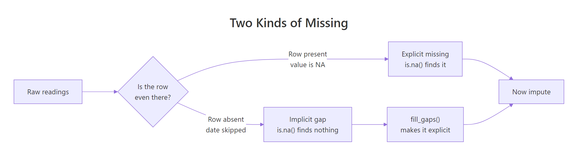
Figure 1: An absent row and an NA are both missing data, but only one of them is visible to is.na().
ts() function just numbers the values one after another, so ten calendar days collapse into six evenly spaced periods and every date after the first gap is silently shifted. Regularise the index first, then convert. The tsibble tutorial covers index handling in more depth.With every gap now visible, the second question is how long the gaps are. A dozen scattered single-month dropouts and one twelve-month outage need completely different treatment, even though sum(is.na(x)) reports the same total for both. rle() compresses a logical vector into runs, which is exactly the summary you want.
Read that as: seventeen isolated single-month gaps, three two-month gaps, and one run of thirteen consecutive months. The thirteen is our twelve-month outage plus one scattered dropout that happened to land right beside it. That single long run is the reason a method that handles the seventeen easy gaps beautifully can still ruin the series.
The third question is whether the gaps cluster anywhere meaningful. To ask that of monthly data you need each gap's calendar month, and cycle() gives it: on a monthly ts object it reports each observation's position within its season, returning 1 for every January through 12 for every December. Indexing month.abb by those positions turns them into month names, and table() counts the ones that landed on a gap.
Nothing dramatic here, which is what we expect since we generated the scattered gaps at random. February looks slightly heavy at six, but with thirty-six gaps spread over twelve months that is ordinary noise. The reason to run this check is the case where it is not noise, and that brings us to why the gaps went missing in the first place.
Statisticians sort missing data into three mechanisms. Translated into time series terms, they look like this.
| Mechanism | In time series terms | Example | Can you impute it? |
|---|---|---|---|
| Missing completely at random | Dropouts unrelated to time or value | Radio packet lost | Yes, safely |
| Missing at random | Dropouts tied to a known feature of the calendar | Store shut on public holidays | Yes, if you model the calendar feature |
| Missing not at random | Dropouts tied to the value that would have been recorded | Sensor saturates and fails above 40 degrees | No, imputation pulls extremes toward the middle |
The third row is the dangerous one and it is very common in sensor data. If a meter cuts out precisely when readings run high, then every gap hides a high value, and any method that interpolates between neighbours will guess something moderate. You will not see the error in a residual plot, because the true values were never recorded. The only defence is knowing your instrument.
Try it: Add a seventh reading on 14 March 2024 with a level of 7.2 to readings, rebuild the tsibble, and count the gaps again. How many gaps are there now, and how long is the new one?
Click to reveal solution
Explanation: Adding a later date extends the range the tsibble considers, so the three days between 10 March and 14 March become a third gap. Adding one observation revealed three absences, which is a good reminder that a gap only exists relative to a defined start and end.
Which simple fills work, and where do they break?
Four repairs cover most of what people reach for. Carry the last value forward, carry the next value back, draw a straight line between the neighbours, or fit a curve through them. The zoo package provides all four, and the fastest way to understand them is to watch them work on seven numbers rather than 240.
Our toy series is deliberately uneven: it climbs gently from 10 to 16, then jumps to 25, then to 50.
Four different answers for the same two holes. na.locf() holds 10 flat until real data returns, which produces a staircase. Setting fromLast = TRUE reverses it into next observation carried backward, which jumps to 16 immediately. na.approx() draws the straight line most people picture when they say interpolation, landing on 12 and 14.
Now look at the spline row, and specifically at the 7.92. The observed series never goes below 10, yet the spline invented a value beneath its own minimum. Splines fit a smooth curve through the surrounding points, and when the series bends sharply, as ours does at the jump to 50, the curve overshoots on the way in. That is the standing risk with na.spline(): it is the most flexible option and the one most willing to produce values your process could never generate.
range() of a spline-filled series before using it.Watching the mechanics is one thing. Scoring them is another, and because we hid the true values ourselves, we can score them exactly. Root mean squared error over just the imputed positions tells us how far each method landed from the truth, in degrees.
Every method beats the mean fill, and the ranking runs from 9.31 degrees down to 6.56. But hold the celebration, because even the best of these is off by six and a half degrees on average, on a series whose entire annual range is about twenty-five degrees. Something is badly wrong, and it is the thirteen-month run we found earlier. We will fix that in the next section.
First, there is a subtler problem that accuracy alone will not reveal. Recall that the whole reason to care is autocorrelation. Mean filling pushed it down. What does interpolation do to it? To isolate the effect, here is a fresh copy of the series with thirty-six scattered gaps and no long run at all.
The two methods fail in opposite directions. Mean filling does what it did in the first section, dragging autocorrelation down at every lag: 0.664 against a true 0.808 at lag 1, and 0.711 against 0.884 at lag 12. Linear interpolation does the reverse at lag 1, returning 0.820 against a true 0.808, and that direction is the new result here. An interpolated point lies exactly on the straight line joining its two neighbours, so it resembles them more closely than a real observation ever would, and the series comes out looking smoother than it is.
Both distortions matter, and they matter in different ways. A depressed autocorrelation makes a series look noisier than it is and pushes model selection toward simpler models. An inflated one makes it look smoother and more predictable than it is, which produces forecast intervals that are too narrow. If your next step is reading an ACF and PACF plot to choose model orders, both errors land directly on that decision.
The last simple tool is a guard rail rather than a method. Every zoo fill accepts maxgap, which sets the longest run it is willing to bridge. Anything longer is left as NA.
The thirteen-month run stayed untouched, and on the gaps it did agree to fill, linear interpolation scored 2.577 degrees instead of 7.524. That is the whole lesson of this section in one number: linear interpolation is not a bad method, it was being asked to do something no straight line can do. maxgap lets you use it where it works and forces you to make a deliberate decision everywhere else.
Try it: Rerun the interpolation with maxgap = 1 so that only isolated single-month gaps are filled. How many NA values survive, and how many were filled?
Click to reveal solution
Explanation: Exactly the seventeen single-month gaps from the rle() profile got filled. The nineteen survivors are the three two-month gaps plus the thirteen-month run, which matches the gap-length table precisely.
How do you fill a gap without erasing the season?
We know why the long outage defeats every method so far. A straight line across twelve months replaces an entire annual cycle with a gentle slope. No interpolation of the raw values can avoid this, because the information needed to fill a January is not in the surrounding months at all. It is in the nineteen other Januaries in the series.
That points straight at the fix. Split the series into a seasonal part and everything else, interpolate only the part that has no pattern, then put the season back. This is exactly what seasonal decomposition gives you, and na.interp() from the forecast package does the whole sequence in one call. It runs an STL decomposition on the observed data, interpolates the seasonally adjusted series, then adds the seasonal component back onto the filled points.
For that to work the function has to know the seasonal period, which means handing it a ts object with the right frequency rather than a bare vector.
From 7.524 degrees down to 2.182, on identical gaps. That is not a tuning improvement, it is a different class of answer, and it comes entirely from telling the method that the series repeats every twelve months.
The month-by-month view of the outage shows where the gain came from.
The linear column drifts from 41.6 down to 38.9 and never leaves the low forties. It claims that year had a January in July. The na.interp column runs 40.6, 42.0, 46.7, 52.5, up to 62.3 in July and back down to 40.2 in December. It reconstructed a summer, because the other nineteen summers in the record told it what one looks like.
Try it: Prove that the frequency is doing the work. Build a ts object from gapped with frequency = 1, so R believes there is no season, run na.interp() on it, and compare the error to the version that knows about the twelve-month cycle.
Click to reveal solution
Explanation: With no seasonal period declared there is nothing to decompose, so na.interp() falls back to plain linear interpolation and reproduces the 7.524 exactly. The entire improvement came from the frequency argument, not from the function name.
Can a model tell you how unsure each filled value is?
Every method so far returns a single number per gap, and that number then sits in your data looking exactly like an observation. A value you invented and a value you measured are treated identically by everything downstream, which is a real problem when a quarter of a year was invented.
A state-space model handles this differently. It treats the series as driven by hidden components you never observe directly, in this case a slowly moving level and a repeating seasonal pattern, plus measurement noise on top. StructTS() estimates those components, and type = "BSM" asks for the basic structural model, the version that carries three hidden components: a level, a slope, and a season. The Kalman smoother then works out the most likely value of each hidden component at every time point, using the whole series, and reports how uncertain it is about each one. Where data exists, the uncertainty is small. Where data is missing, it grows.
Filling a gap means adding the smoothed level and the smoothed seasonal component at that time point. KalmanSmooth() returns the smoothed components as columns of sm$smooth, in the order level, slope, season, so the two we want are columns 1 and 3.
The structural model scored 2.884 against 2.182 for na.interp. It lost. That result is worth sitting with, because state-space methods carry a reputation as the sophisticated option, and on this series the simpler seasonal decomposition was more accurate. Sophistication is not accuracy, and the only way to know which wins on your data is to measure, which is the subject of the next section.
What the state-space model does give you, and no interpolation can, is a per-point measure of its own uncertainty. The smoother's variance output tells you how confident it is about the level and season at each time point. sm$var holds one variance matrix per time point, so sm$var[, 1, 1] is the variance of the level and sm$var[, 3, 3] the variance of the season. Add the two and take the square root and you have a standard error in degrees.
The pattern is exactly what intuition demands. At an observed month the standard error is 1.66 degrees, which is just the model's measurement noise. At an isolated one-month gap it rises to 2.87, because the value is inferred from neighbours rather than measured. At the start of the long outage it is 3.74, and six months in, as far from real data as you can get, it reaches 4.55.
That is a real, usable number. It tells you that the mid-outage estimates deserve roughly three times the doubt of an observed month, and it gives you grounds to widen a downstream interval or to exclude those months from an evaluation. Every other method in this tutorial reports the same confidence for a value squeezed between two neighbours and a value invented in the middle of a year-long blackout.
The imputeTS package packages these approaches behind a consistent interface, along with the best gap diagnostics available anywhere. It is not part of the interactive environment here, so run this one locally, in a session where gapped, temps and holes from the blocks above already exist.
# Run this locally in RStudio: install.packages("imputeTS") first.
gts_static <- ts(gapped, start = c(1920, 1), frequency = 12)

profile <- imputeTS::statsNA(gts_static, print_only = FALSE)
c(missing = profile$number_NAs, gaps = profile$number_na_gaps,
  longest_gap = profile$longest_na_gap, commonest_gap = profile$most_frequent_na_gap)
#>       missing          gaps   longest_gap commonest_gap
#>            36            21            13             1

profile$percentage_NAs
#> [1] "15%"

round(c(na_interpolation = rmse(imputeTS::na_interpolation(gts_static), temps, holes),
        na_seadec        = rmse(imputeTS::na_seadec(gts_static),        temps, holes),
        na_kalman        = rmse(imputeTS::na_kalman(gts_static, model = "StructTS"), temps, holes)), 3)
#> na_interpolation        na_seadec        na_kalman
#>            7.524            2.188            2.944
Those three numbers should look familiar. na_interpolation reproduces the linear result to three decimals, na_seadec lands within 0.006 of na.interp, and na_kalman matches the structural model we built by hand. The package is a convenience layer over the same mechanics, which is worth knowing because it means the reasoning transfers: understanding why seasonal decomposition beat interpolation here tells you why na_seadec will beat na_interpolation on your data too.
imputeTS last and use zoo::na.locf() explicitly, or skip the attach and call imputeTS::na_kalman() with the prefix as shown above. Older tutorials also use dot names like na.kalman and plotNA.distribution, which were replaced by na_kalman and ggplot_na_distribution in version 3.0.Try it: The thirteen-month run in this series covers indices 121 to 133. Read the smoother's standard error at the first month of the run, the seventh, the thirteenth, and the first observed month afterwards. Does the uncertainty peak where you expect?
Click to reveal solution
Explanation: Uncertainty climbs to a peak of 4.56 in the middle of the run, where the smoother is furthest from real data in both directions, then falls back as it approaches the observations on the far side. The first observed month afterwards drops to 2.37, still above the 1.66 of a month deep inside clean data, because the smoother is partly reconstructing that neighbourhood too.
How do you prove which method is best for your series?
Three sections have now produced three different winners. Spline led among the simple fills, na.interp beat everything on the long outage, and the structural model came third despite being the most elaborate. There is no ranking that holds across series, and there is no ranking that even holds across different gap patterns in the same series.
The way out is the same trick we have been using implicitly all along: hide values you already know, fill them, and score the answers. This works on any real series, because there is always a stretch of complete data to hide values from. No ground truth needed beyond the data you already have.

Figure 2: Hide values you already know, then score every candidate method against them.
Here is the harness. It takes a complete series plus a logical mask of positions to hide. It blanks those positions, then reports how far each of four methods landed from the values it hid.
With thirty scattered single-month gaps the four methods finish close together. na_interp wins at 2.605, linear is barely behind at 2.827, and even carrying the last value forward only costs 5.479. When gaps are isolated, the choice of method is a minor decision.
Now change one thing. Same series, same number of methods, but the missing values sit in one block of eighteen consecutive months.
The winner did not change, but everything behind it did. na_interp barely moved, from 2.605 to 2.856. Every other method got several times worse. Linear quadrupled to 10.570, and spline went from second-best at 3.051 to worst by a wide margin at 19.542, because an unconstrained curve fitted across eighteen months goes wherever the polynomial takes it.
One mask could be luck, so repeat it. Twenty random twelve-month outages at different positions in the series, averaged.
The result is stable. Across twenty different outage positions na_interp averages 2.928 degrees while everything else sits above eleven. For this series with gaps of this shape, the decision is not close, and now you have evidence rather than a rule of thumb.
Try it: Add mean filling to the comparison so you can see how far ahead of the baseline the good methods really are on a long block. Write a small scoring function containing just mean fill and na.interp, and run it on block_mask.
Click to reveal solution
Explanation: Mean filling scores 9.710 on the block, which is better than spline at 19.542 and roughly on par with locf and linear. That is a genuinely uncomfortable result: three methods that look far more principled than painting the average across a gap did not actually beat it here, because none of them knows about the season either.
When should you skip imputation, and how do you avoid leaking the future?
There is an assumption buried in everything above: that you need complete data before you can model. For a large family of models that assumption is simply false, and acting on it makes your results worse rather than better.
ARIMA models are estimated through a Kalman filter, and the filter has a built-in rule for a missing observation: skip the update step and carry the prediction forward. Missing values are handled exactly, as part of the likelihood, with no filling required. Watch what happens to the estimated noise variance when you impute first instead.
The complete series, the truth, gives a noise variance of 10.644. Fitting to the gappy series gives 9.444, a mild underestimate. Fitting to the imputed series gives 8.723, the furthest from the truth of the three.
Think about what that means. Imputing made the model more confident than the complete data would justify. The filled values sit on a smooth reconstruction with no noise of their own, so the model sees a tidier series than reality and shrinks its error variance to match. Every prediction interval built on that fit will be too narrow, and the more you impute the more confident and the more wrong it gets.
If you want the model's own estimate of the missing values, ask it directly. In fable, interpolate() returns the fitted model's best guess at each gap.
ARIMA() selected a seasonal model on its own and interpolated to within 2.260 degrees, essentially tying with na.interp. The difference is that this estimate is internally consistent with the model you are going to forecast from, rather than being produced by a separate procedure and then handed over as if it were data.
Not every model is so accommodating, and the failure can be silent. Exponential smoothing has no equivalent way to skip a missing observation, so gaps do not throw an error, they change what gets fitted.
On complete data ETS() selects (A,N,A): additive error, no trend, additive season. On the same series with fifteen percent missing it selects (M,N,N), which has no seasonal component at all. Nothing warned us. A model of monthly temperature that does not know about summer will forecast a flat line, and the only visible symptom is a model specification you would have to be paying attention to notice.
That leads to the last trap, and it is the one that silently inflates backtest results. Look again at how these methods work. Linear interpolation reads the next observed value. na.interp decomposes the entire series. The Kalman smoother explicitly uses observations from both directions. All of them are two-sided by construction.
For describing history that is a strength, since more information gives better estimates. For evaluating a forecast it is cheating, because at the moment you were forecasting, the future values those methods used had not happened yet.
Two-sided interpolation looks twice as accurate. It is not twice as clever, it just had twice the information, half of which was unavailable at the time. Here is a single gap to make that concrete.
At index 31 the truth is 56.80. Carrying the previous value forward gives 57.80, using only the past. Linear interpolation gives 56.05, and it landed closer because it averaged toward 54.30, the value at index 32, a month that had not occurred yet. Its accuracy is borrowed from the future.
The rule is simple once the distinction is clear. For describing, cleaning or charting a historical series, two-sided methods are correct and you should use the best one you can find. For anything evaluated as a forecast, impute using only data available at the forecast origin, which means one-sided methods or a Kalman filter run in filtering mode rather than smoothing mode.
Try it: Confirm that arima() really did use only the observed months. Fit the model to gapped_ts and report how many months the series contains against how many were actually observed, then look at the estimated coefficients.
Click to reveal solution
Explanation: The model fitted happily to 204 observations spread across 240 time points, and it recovered a strong seasonal autoregressive coefficient of 0.885. No imputation was involved at any stage. The ARIMA tutorial covers what these coefficients mean.
Complete Example
Here is the whole workflow on one series: regularise the index, make gaps explicit, mark which values are invented, then fill with a method chosen for the gap profile.
Five steps, and the fourth is the one people skip. fill_gaps() guarantees no absence stays invisible. The imputed flag is computed before filling, so it records the truth about the original data, and it travels with the series from then on. Later you can exclude invented points from an accuracy calculation, colour them differently in a chart, or feed the flag to a model as a regressor. Once the values are filled and the flag is gone, no one downstream can tell measurement from reconstruction.
Frequently Asked Questions
What is the best imputation method for time series? There is no fixed answer, and the mask-and-score harness above exists precisely because of that. As a starting point: for scattered gaps much shorter than one seasonal period, linear interpolation via na.approx() is hard to beat. For gaps approaching or exceeding one seasonal period, use a seasonal method such as forecast::na.interp() or imputeTS::na_seadec(). In the twenty-outage test here the seasonal method averaged 2.928 degrees against 11.9 for linear.
What is the difference between na.approx() and na.locf()? na.locf() carries the last observed value forward, producing flat steps and using only past information. na.approx() draws a straight line between the observations either side, which is more accurate for describing history but uses future values. That difference matters when the imputed series feeds a backtest.
Can I use mean imputation for time series data? Only as a deliberate baseline. Mean filling shrinks the variance and pushes autocorrelation down at every lag, which biases model selection and forecast intervals. In the first example it dropped the lag-12 autocorrelation from 0.884 to 0.729.
What does maxgap do in na.approx()? It sets the longest run of consecutive NA values the function will bridge. Longer runs are left as NA so you have to decide about them explicitly. Setting maxgap = 3 on the example series improved the error on filled gaps from 7.524 to 2.577 by simply declining the impossible ones.
Does ARIMA handle missing values automatically? Yes. Both stats::arima() and fable::ARIMA() evaluate the likelihood through a Kalman filter, which skips the update step at a missing observation. Imputing first is not required and makes the estimated noise variance too small, as shown above. fable::interpolate() returns the model's own estimate of the gaps if you want the values.
Which forecasting models can handle NA values in R? In fable, ARIMA, dynamic regression, NNAR and the naive benchmarks tolerate missing values. ETS and STL do not, and ETS fails quietly by selecting a non-seasonal specification rather than raising an error.
How much missing data is too much for imputation? The total percentage matters much less than the shape. Twenty percent scattered across isolated points is routine. Five percent concentrated in one block spanning a full season may be unrecoverable, because no information about that stretch survives. Profile the gap lengths with rle() before judging.
Is forward fill or backward fill better for time series? Forward fill, in almost every case. Backward fill takes a value from the future and writes it into the past, which corrupts any evaluation that respects time order. Use backward fill only for a leading NA at the very start of a series, where no earlier value exists.
Can mice be used for time series data? Not usefully on a single series. Multiple imputation methods like mice exploit correlations between variables, and a univariate series has none to exploit. The information lives in the time dimension instead, which is what the methods in this tutorial use. For missing values in ordinary cross-sectional data, see the general missing value tutorial.
Practice Exercises
Exercise 1: Profile a gap pattern, then choose from the profile
Generate a mixed gap pattern on temps: eight scattered single-month dropouts somewhere between index 20 and 200, plus one twelve-month block at indices 60 to 71. Use set.seed(505) and sample(20:200, 8). Profile the gap lengths with rle(), then score all four methods and check that your profile predicted the winner.
Click to reveal solution
Explanation: The profile shows eight one-month gaps and one twelve-month run, and that single long run decides everything. na_interp wins at 2.914 while the others sit between 9.1 and 15.5. The eight easy gaps are filled well by every method, but the twelve-month block dominates the error, so the presence of one long run is enough to settle the choice.
Exercise 2: Extend the harness and vary the missingness rate
Write a scoring function with three methods: next observation carried backward (na.locf with fromLast = TRUE), linear interpolation, and na.interp. Score it at two rates of scattered missingness, 12 points and 60 points, both sampled from indices 13 to 228 with set.seed(31). Present the result as a two-row matrix.
Click to reveal solution
Explanation: The ranking flips between the two rates. At five percent missing, linear wins at 2.531 because gaps are isolated and neighbours are close. At twenty-five percent, gaps start clumping into runs of two and three, neighbours drift further apart, and the seasonal method takes over at 2.632. A method chosen at one missingness rate is not automatically right at another.
Exercise 3: Build the honest comparison against the leaky one
Set a forecast origin at index 180. Impute the history two ways: honestly, using na.locf() on gapped[1:origin] only, and leakily, by interpolating the full 240-month series and then taking the first 180 values. Score both on the scattered gaps within the history, excluding indices 118 to 135 so the long outage does not dominate. Report the two errors.
Click to reveal solution
Explanation: The leaky version scores 2.226 against 5.559, so it looks two and a half times better. That gap is not skill, it is the amount of future information that flowed into the past. If you fill the whole series before splitting, this is the size of the illusion baked into your backtest, and it will not reproduce when the model meets data that has not happened yet.
Summary
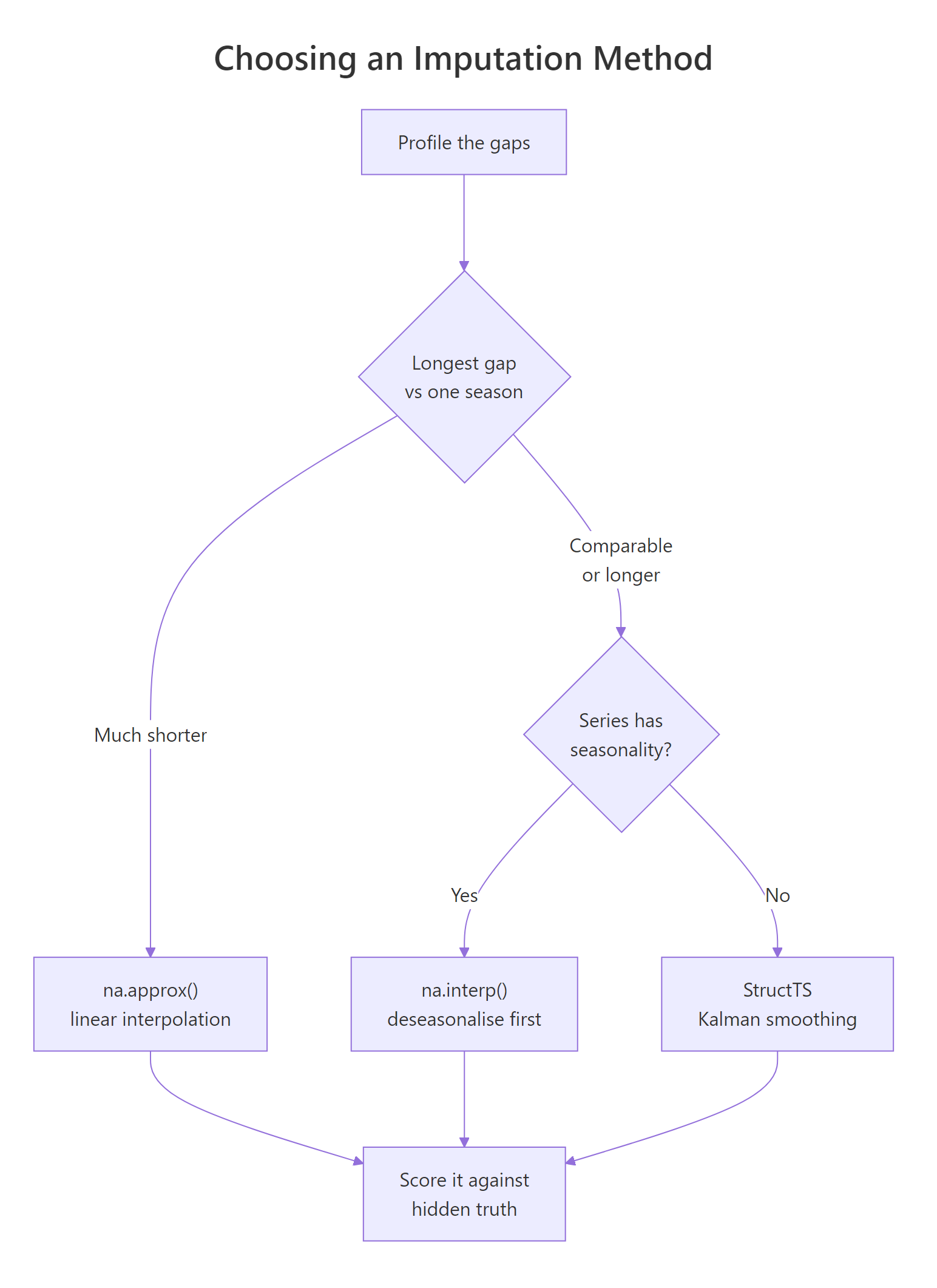
Figure 3: Gap length relative to one seasonal period is the variable that decides the method.
| Method | Function | Wins when | Fails when |
|---|---|---|---|
| Mean fill | x[is.na(x)] <- mean(...) |
Never, except as a baseline | Always; it flattens the season and shrinks autocorrelation |
| Carry forward | zoo::na.locf() |
You need a one-sided fill for a backtest | Gaps are long; it produces flat steps |
| Linear | zoo::na.approx() |
Gaps are short relative to the season | Gaps span a seasonal cycle |
| Spline | zoo::na.spline() |
The series curves smoothly and gaps are short | Long gaps; it overshoots outside the observed range |
| Seasonal decomposition | forecast::na.interp() |
The series is seasonal, at any gap length | The series has no seasonal structure to exploit |
| State space | StructTS() plus KalmanSmooth() |
You need per-value uncertainty | You need the single most accurate point estimate |
| No imputation | arima(), fable::ARIMA() |
The model handles NA natively | The model family is ETS or STL |
The workflow that holds regardless of series:
- Make every gap visible with
fill_gaps()before you count anything. - Profile gap lengths with
rle(), and compare the longest run to one seasonal period. - Ask why the data is missing. Missingness tied to the value itself cannot be safely imputed.
- Hide known values and score the candidates. Let the numbers pick the winner.
- Keep a flag column marking which values were invented.
- If the model handles missing values natively, consider not imputing at all.
- For anything evaluated as a forecast, impute inside the fold using only the past.
References
- Hyndman, R.J. and Athanasopoulos, G. Forecasting: Principles and Practice, 3rd edition, section 13.9 on outliers and missing values. Link
- Moritz, S. and Bartz-Beielstein, T. imputeTS: Time Series Missing Value Imputation in R. The R Journal 9(1), 2017. Link
- Moritz, S. et al. Comparison of different methods for univariate time series imputation in R. arXiv:1510.03924. Link
- tsibble reference: handling implicit missing values. Link
- zoo reference:
na.approxandna.spline. Link - forecast reference:
na.interp. Link - R Core Team.
StructTSand Kalman filtering reference. Link - imputeTS package documentation, current API. Link
Continue Learning
- tsibble in R covers index handling, keys and gap detection in depth, and is the natural companion to the
fill_gaps()work here. - Missing Values in R handles the cross-sectional case, where correlations between columns do the work that time dependence does here.
- Time Series Cross-Validation in R shows the fold structure that imputation must live inside if your backtest scores are going to mean anything.