Dynamic Regression in R: Regression with ARIMA Errors
Dynamic regression is a forecasting model that pairs an ordinary regression on outside predictors with ARIMA-modeled errors. In R you fit one by passing your predictors to the xreg argument of auto.arima() from the forecast package, which keeps your estimates honest where an ordinary regression would mislead.
Why does ordinary regression fail on a time series?
Linear regression is the first tool most people reach for when one thing might explain another. On time series data it has a serious flaw: it reports strong relationships that are not real. Before we build anything, let's see the problem for ourselves on data where we already know the right answer.
Here is the trap in eight lines. We create two series that have absolutely nothing to do with each other. Each one is a random walk: it starts at zero and takes random steps, like a coin-flip stroll. They are generated from separate random numbers, so any link between them is pure chance. Then we regress one on the other and read the result.
Look at the walk_x row. The slope is 1.13, its t value is 22.24, and the p value is 0.0000. In any statistics class, those numbers say the effect is real and "highly significant." Yet we know the truth, because we built the data. There is no relationship at all. The regression is confidently describing a link that does not exist.
The R-squared makes it worse. It tells you what fraction of the movement in one series the other appears to explain.
An R-squared of 0.714 says walk_x explains 71% of walk_y. That would be an excellent model in any other setting. Here it means nothing. This failure has a name, spurious regression, and it happens because both series drift over time, so they often wander in loosely similar ways and look related purely by chance.
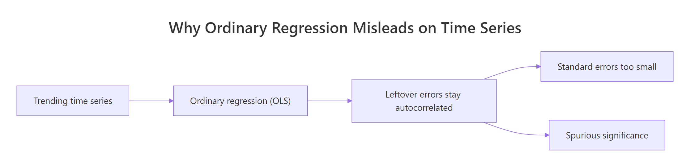
Figure 1: How autocorrelated errors let ordinary regression report spurious significance and understated standard errors.
The root cause is the regression's errors. Ordinary regression assumes its leftover errors are independent, one observation telling you nothing about the next. In a time series that assumption is almost never true: today's value is close to yesterday's, so the errors are autocorrelated. When the errors carry that hidden time structure, the significance test counts the same information many times over and reports far more certainty than it has earned.
Try it: A different starting seed gives a different pair of unrelated walks, and the fake relationship shows up again. Run this and read the t value.
Click to reveal solution
Explanation: Two brand new unrelated walks, and the slope is again "significant" at a p value of 0.0003. Spurious regression is not a one-off fluke of one seed, it is what ordinary regression does to trending series in general.
What is dynamic regression, and how does it fix this?
Dynamic regression fixes the trap without throwing away the regression you wanted in the first place. The idea is to give the model two jobs instead of one. The regression part still estimates how the predictor affects your series. A second part, an ARIMA model, is added to soak up the leftover time structure in the errors, so the errors the regression sees are finally the independent noise it always assumed.
That is why the honest name for this model is "regression with ARIMA errors." Written out, it is an ordinary straight-line regression where the error term is not plain noise but follows its own ARIMA process.
$$y_t = \beta_0 + \beta_1 x_t + n_t$$
Where:
- $y_t$ is the value of your series at time $t$
- $\beta_0$ is the intercept, the baseline level
- $\beta_1$ is the effect of the predictor, the number you usually care about
- $x_t$ is the predictor at time $t$
- $n_t$ is the error, which follows an ARIMA model instead of being independent noise
That last line is the whole trick. In an ordinary regression, $n_t$ is assumed independent. Dynamic regression lets $n_t$ carry the autocorrelation that time series always have, so the ARIMA part explains the memory and the regression part is left with an honest effect. If the math is not your thing, skip it: the practical point is that R handles $n_t$ for you.
Let's hand the exact same two random walks to a dynamic regression and see the fake relationship disappear. We use auto.arima() and pass the predictor through the xreg argument. That single argument is what turns auto.arima() from a plain forecaster into a dynamic regression.
Read the xreg coefficient: 0.0107, with a standard error of 0.0639. The effect is smaller than its own standard error, meaning it is statistically indistinguishable from zero. The verdict flipped completely. Ordinary regression said 1.13 and "highly significant." Dynamic regression, once it accounts for the time structure, says "no reliable effect here." That is the correct answer, because we built the two series to be unrelated.
Notice the label R printed, "Regression with ARIMA(0,1,1) errors." The (0,1,1) is the ARIMA model chosen for the errors, and the 1 in the middle is the key. It means the errors were differenced once, which is how the model stripped out the drift that fooled ordinary regression. We will unpack that middle number shortly.
xreg itself, ARIMAX in R is the companion to this page, which focuses on why dynamic regression matters.Try it: A quick way to judge an effect is its t ratio, the coefficient divided by its standard error. A value near zero means "no signal." Compute it for the xreg coefficient above.
Click to reveal solution
Explanation: A t ratio of 0.168 is nowhere near the rough threshold of 2 that signals significance. Dynamic regression correctly reports the predictor as useless, exactly the opposite of the ordinary regression's t value of 22.
How do you fit a dynamic regression in R?
Killing false signals is only half the value. Dynamic regression also measures real effects correctly, giving you the right slope with trustworthy uncertainty. To show this, we need data where a genuine relationship exists, so let's build one on purpose.
Imagine a business tracking daily signups against how much it spends on ads. We make signups genuinely depend on ad spend: each unit of spend truly adds 1.5 signups, and we bury that signal under autocorrelated noise so it behaves like a real, sticky series. Because we set the true effect ourselves, we know a good model should recover a slope near 1.5.
Ordinary regression estimates the slope at 1.5335, close to the true 1.5. So the point estimate is fine. The problem hides in the Std. Error column, 0.0699. Because the errors here are autocorrelated, that standard error is too small, and every conclusion about significance built on it is overconfident. Now fit the dynamic regression on the same data and watch the standard error tell the truth.
The slope is 1.6057, again near the true 1.5. The model also found ar1 of 0.56, which is the autocorrelation in the errors that ordinary regression ignored. The interesting comparison is the two standard errors side by side.
cbind(ad_spend = ad_spend) instead of a bare vector labels the coefficient ad_spend in the printout rather than the generic xreg, which pays off once you have several predictors to tell apart.The dynamic-regression standard error, 0.0893, is about 28% wider than the ordinary 0.0699. Both models agree the effect is near 1.5, but they disagree about how sure we should be. Ordinary regression treated 180 autocorrelated points as if they carried more independent evidence than they really do, so it understated the uncertainty. The dynamic regression gives the same slope with an honest margin around it.
You do not have to let auto.arima() pick the error structure. When you want a specific ARIMA order, Arima() takes an order argument and the same xreg. Fitting the (1, 0, 0) structure by hand reproduces the automatic model exactly.
xreg must be the predictor at the same time as the first value of your series, and missing values will break or bias the fit. Align by date and fill or drop NA values before fitting.The output is identical, which confirms auto.arima() chose (1, 0, 0) for us. In practice, let it choose unless you have a reason not to.
Try it: Pull the honest standard error of the ad_spend effect straight from the fitted model. This is the number you would report.
Click to reveal solution
Explanation: The vcov() function returns the model's variance-covariance matrix; the square root of its diagonal gives each coefficient's standard error. For ad_spend that is 0.0893, the trustworthy figure to quote rather than the ordinary regression's 0.0699.
Why must the ARIMA errors be stationary?
You may have noticed the two models chose different middle numbers. The random-walk model differenced its errors, ARIMA(0,1,1), while the signups model did not, ARIMA(1,0,0). That middle number, the number of differences, is where dynamic regression does its most important work, so it is worth understanding.
Differencing means replacing each value with the change from the previous value. It exists to make a series stationary, meaning its behaviour, its average level and its swings, stays steady over time instead of drifting. Dynamic regression needs the ARIMA error to be stationary. When your series trends, the leftover error trends too, so auto.arima() differences it away by choosing a middle number of 1. That single step removes the shared drift that caused the spurious result in the first place.
R has a helper that reports how many differences a series needs. Run it on the random walk from the start of this tutorial.
The answer is 1, which is exactly the middle number the dynamic regression chose for that series. This is not a coincidence: auto.arima() runs this same check internally and differences the errors accordingly. To see that differencing is what defused the spurious link, we can do it by hand. Regressing the change in one walk on the change in the other should show no relationship.
The slope is now -0.0020 with a p value of 0.9753, as unrelated as it should be. Differencing by hand reached the same honest verdict that dynamic regression reached automatically. The lesson is that the drift, not any true link, drove the original 1.13 slope, and removing the drift removes the illusion.
auto.arima(); it detects the need, differences the series and its errors together, and reports the middle number so you can see it happened.Try it: The honest signups series was built to be stationary, so it should need no differencing at all. Confirm it.
Click to reveal solution
Explanation: The answer is 0, so no differencing is needed, which matches the ARIMA(1,0,0) the model chose. A stationary series keeps its middle number at 0; a drifting one gets differenced. Dynamic regression adapts to whichever you have.
How do you check the model and forecast?
Two jobs remain before you trust a dynamic regression: confirm the model is adequate, then forecast with it. Both are quick, and both have a catch worth knowing.
Checking the model means confirming the errors are finally white noise, plain random static with no leftover pattern. If any structure remains, the ARIMA part did not fully do its job. The checkresiduals() function runs a Ljung-Box test, where a p value above 0.05 means the residuals look like clean noise.
The p value is 0.5866, comfortably above 0.05, so the residuals pass. The autocorrelation the ordinary regression left behind has been absorbed by the ARIMA part, and what remains is the independent noise the regression needs. This diagnostic is your proof that the standard errors can be trusted.
Now forecasting, and here is the catch. A dynamic regression cannot forecast on its own, because it needs the future values of its predictors. To predict signups next month, you must first tell the model what ad spend will be next month. You pass those future values through the same xreg argument, and the horizon is simply however many rows you supply.
Each row is one future month. The Point Forecast is the single best guess, and the interval columns give ranges: the model is 80% sure the value falls between Lo 80 and Hi 80, and 95% sure between Lo 95 and Hi 95. The forecasts rise and fall because the future ad spend we supplied rises and falls, and the slope of 1.6 carries that pattern into signups. A picture makes it clearer, and autoplot() draws the history and forecast together.
Try it: Forecast a shorter horizon by supplying only 6 future values. The horizon follows the number of rows you pass.
Click to reveal solution
Explanation: Six future values means a six-row forecast. There is no separate horizon setting to remember; the number of rows in xreg is the horizon.
Complete Example: A real relationship that survives
The random walks were rigged to show a fake relationship collapse. Real economic data is more interesting: sometimes the relationship is genuine, and dynamic regression confirms it while ordinary regression exaggerates it. Let's test a real question on real numbers. Does the personal savings rate move consumer spending? Common sense says when people save a larger share of income, they spend a smaller one, so we expect a negative link.
The built-in economics dataset carries decades of monthly US figures, including pce (personal consumption expenditure, in billions of dollars) and psavert (the personal savings rate, in percent). We start with the naive approach, an ordinary regression of spending on the savings rate, and then inspect its residuals.
Ordinary regression reports a slope of -951, meaning each extra percentage point of savings rate is tied to $951 billion less spending, with a t value of -31. That is enormous and, taken at face value, decisive. But we have learned to be suspicious, so we check whether the residuals are autocorrelated, which would sink those standard errors.
The first value is always 1, the residual's correlation with itself, so ignore it. The next values, 0.940 and 0.905, are enormous. The residuals are almost perfectly autocorrelated, which is a strong warning that the -951 slope is inflated by the shared trend of the two series, not a clean relationship. This is the same spurious regression from the opening, now inside real data, and dynamic regression fixes it here too.
The model chose ARIMA(1,1,2) errors, so it differenced once to remove the shared trend. The honest xreg coefficient is -11.64, with a standard error of 1.25, giving a t value near -9. The relationship is real and clearly significant, but it is roughly 80 times smaller than the -951 ordinary regression claimed. Most of that giant number was the trend both series happened to share, not a true effect of saving on spending. Before quoting the number, confirm the residuals are clean.
The Ljung-Box p value is 0.1907, above 0.05, so the residuals pass as white noise and the standard error can be trusted. Finally, pull the coefficient out for reporting.
The pairing tells the whole story of this tutorial. A fake relationship, the two random walks, collapses to nothing under dynamic regression. A real relationship, savings against spending, survives but shrinks to its honest size. Ordinary regression cannot tell those two situations apart. Dynamic regression can.
Frequently Asked Questions
What is dynamic regression in one sentence? It is a linear regression whose error term is modeled as an ARIMA process, so the regression measures a predictor's effect while the ARIMA part absorbs the time structure that would otherwise corrupt the result.
How is it different from ARIMAX or "ARIMA with xreg"? In R's forecast package they use the same machinery: you pass predictors to xreg in Arima() or auto.arima(). "ARIMAX" usually emphasizes the mechanics of adding regressors to a forecaster, which ARIMAX in R covers in depth. This page emphasizes the why: dynamic regression is the principled framework that keeps regression honest on time series. R prints what it actually fits as "Regression with ARIMA errors."
Why not just use ordinary regression? Because ordinary regression assumes independent errors, and time series errors are autocorrelated. That assumption failure produces spurious significance and standard errors that are too small, as the random-walk example showed. Dynamic regression repairs both problems.
Do I need future values of the predictors to forecast? Yes, and this is the main practical catch. To forecast ahead you must supply the predictors' future values through xreg. If they are known in advance (a budget, a calendar effect) you are safe; if not, you must forecast the predictor first, and its uncertainty flows into your final forecast.
How do I know if I need to difference? You usually do not decide by hand. auto.arima() runs unit-root tests and differences the errors when needed, reporting the choice as the middle number of the ARIMA order. The ndiffs() function shows the same recommendation for a single series if you want to check yourself.
Practice Exercises
These combine ideas from across the tutorial. Each starter block runs as-is, so write your solution and then reveal ours to compare. The exercises use their own variable names so they will not clash with the code above.
Exercise 1: Expose and fix a spurious link
Build two independent random walks of length 250 with set.seed(303). First show that ordinary regression finds a "significant" slope between them, then show that a dynamic regression with xreg neutralizes it.
Click to reveal solution
Explanation: Ordinary regression reports a slope of -1.37 with a t value of -12, apparently rock solid. Dynamic regression shrinks the coefficient to -0.11 against a standard error of 0.06, so it is barely more than one standard error from zero. The "strong" relationship was an artifact of two shared drifts.
Exercise 2: Recover a known effect and prove the model is adequate
Build a series my_y that truly depends on a predictor my_x with a slope of 0.8, plus autocorrelated noise, using set.seed(101) and length 300. Fit a dynamic regression, confirm it recovers the 0.8, and check that the residuals are white noise.
Click to reveal solution
Explanation: The dynamic regression recovers a slope of 0.833, right on top of the true 0.8, and the Ljung-Box p value of 0.3462 confirms the residuals are clean noise. A recovered effect plus a passing residual check is exactly the evidence that your model is trustworthy.
Exercise 3: Earn a second predictor with AICc
Using the economics data, fit a dynamic regression of pce on both psavert and pop (population). Compare its AICc to the single-predictor model dyn_econ from the Complete Example, then read the coefficients. Lower AICc is better.
Click to reveal solution
Explanation: Adding population lowers AICc from 5230.7 to 5216.1, a drop of about 15, so the second predictor earns its place. The savings-rate effect holds steady near -12, while the population coefficient is a small partial effect you should not over-read on its own. Comparing AICc with and without a predictor is how you decide whether to keep it.
Summary
Dynamic regression is ordinary regression made safe for time series. You keep the regression that estimates your predictor's effect, and you add an ARIMA model for the errors so that autocorrelation and trend cannot corrupt the result. In R, one xreg argument turns auto.arima() into exactly this model.

Figure 2: The dynamic regression workflow, from fitting with xreg to forecasting with future predictors.
| Task | How | Key point |
|---|---|---|
| Fit | auto.arima(y, xreg = X) |
The xreg argument makes it a dynamic regression |
| Control the order | Arima(y, order, xreg = X) |
Set the ARIMA order for the errors by hand |
| Handle trend | Nothing extra | auto.arima() differences the errors for you |
| Check | checkresiduals(fit) |
Ljung-Box p above 0.05 means the errors are clean |
| Forecast | forecast(fit, xreg = future_X) |
You must supply future predictor values |
| Read the effect | coef(fit)["xreg"] |
An honest slope with a trustworthy standard error |
Keep these takeaways close:
- Ordinary regression lies on time series. Autocorrelated errors produce spurious significance and standard errors that are far too small.
- Dynamic regression splits the work in two. A regression captures the predictor's effect, and an ARIMA model soaks up the leftover time structure.
- Differencing removes the shared trend.
auto.arima()decides how much to difference and applies it to the series and its errors together, so you never difference predictors by hand. - Always check the residuals. A passing Ljung-Box test is your proof that the standard errors, and therefore your conclusions, can be trusted.
- Forecasting needs future predictors. Unlike a plain ARIMA, a dynamic regression cannot project its own inputs forward.
References
- Hyndman, R.J., & Athanasopoulos, G. - Forecasting: Principles and Practice, 3rd edition. Chapter 10: Dynamic regression models. Link
- Hyndman, R.J., & Athanasopoulos, G. - Forecasting: Principles and Practice, 2nd edition. Section 9.2: Regression with ARIMA errors in R. Link
- Hyndman, R.J., & Khandakar, Y. - "Automatic Time Series Forecasting: The forecast Package for R." Journal of Statistical Software, 27(3), 2008. Link
- Granger, C.W.J., & Newbold, P. - "Spurious regressions in econometrics." Journal of Econometrics, 2(2), 1974. Link90034-7)
- forecast package -
auto.arima()reference. Link - forecast package -
Arima()reference. Link - ggplot2 -
economicsdataset reference. Link
Continue Learning
- ARIMAX in R - the companion page, covering the mechanics of the
xregargument in depth. - ARIMA in R - the foundation this model builds on, covering what AR, I, and MA mean.
- SARIMA in R - the seasonal extension for series with a repeating yearly or weekly pattern.
- ARIMA Diagnostics in R - go deeper on residual checks and the Ljung-Box test used here.
- ACF and PACF in R - the autocorrelation plots behind the residual diagnostics in this tutorial.