ARIMAX in R: ARIMA with External Regressors (xreg)
ARIMAX extends ARIMA by letting the model use outside predictors, like temperature, price, or a promotion flag, alongside a series' own past. In R you fit one by passing those predictors to the xreg argument of Arima() or auto.arima() from the forecast package.
Why add external regressors to an ARIMA model?
A plain ARIMA model forecasts a series using only its own past values and its own past errors. That is powerful, but it is also blind to things you already know. An ice-cream shop's sales climb when the weather is hot. Website traffic jumps during a sale. ARIMA cannot see any of that. ARIMAX can, because the X stands for eXternal: you hand the model one or more outside drivers and it uses them. Let's build a small daily-sales series that genuinely follows temperature, then watch auto.arima() pin the temperature effect down.
First, we create 120 days of data. Sales are built as a baseline of 40, plus 3 units for every degree of temperature, plus some autocorrelated noise so it behaves like a real series. Because we made the data, we know the true answer in advance: the temperature effect is exactly 3.
Each row is one day with a temperature reading and a sales count. Now the payoff. We hand both series to auto.arima() and pass temperature through the xreg argument. The one extra touch is cbind(temperature = temperature), which bundles the regressor into a named column so R labels its coefficient clearly.
Read the coefficient row. The temperature coefficient is 3.0892, right next to the true effect of 3 that we built in. The intercept is 40.26, which recovers the baseline of 40. The ar1 term of 0.50 is the model handling the leftover autocorrelation in the noise. In one line, ARIMAX separated the part of sales that temperature explains from the part that is pure time-series inertia.
xreg argument adds.Notice the label R printed: "Regression with ARIMA(1,0,0) errors," not "ARIMAX." That phrase is the honest description of what R fits, and we will unpack it later. For now, the mental model is simple. A plain ARIMA uses one input, the series itself. ARIMAX adds more input columns.
| Feature | Plain ARIMA | ARIMAX |
|---|---|---|
| Uses the series' own past | Yes | Yes |
| Uses outside predictors | No | Yes, via xreg |
| Good when | The series drives itself | A known factor drives the series |
| Needs future inputs to forecast | No | Yes, future xreg values |
The diagram below shows the same idea as a picture: the series' own AR, I, and MA structure enters the model, the external regressors enter alongside it, and the combined model produces both forecasts and effect estimates.
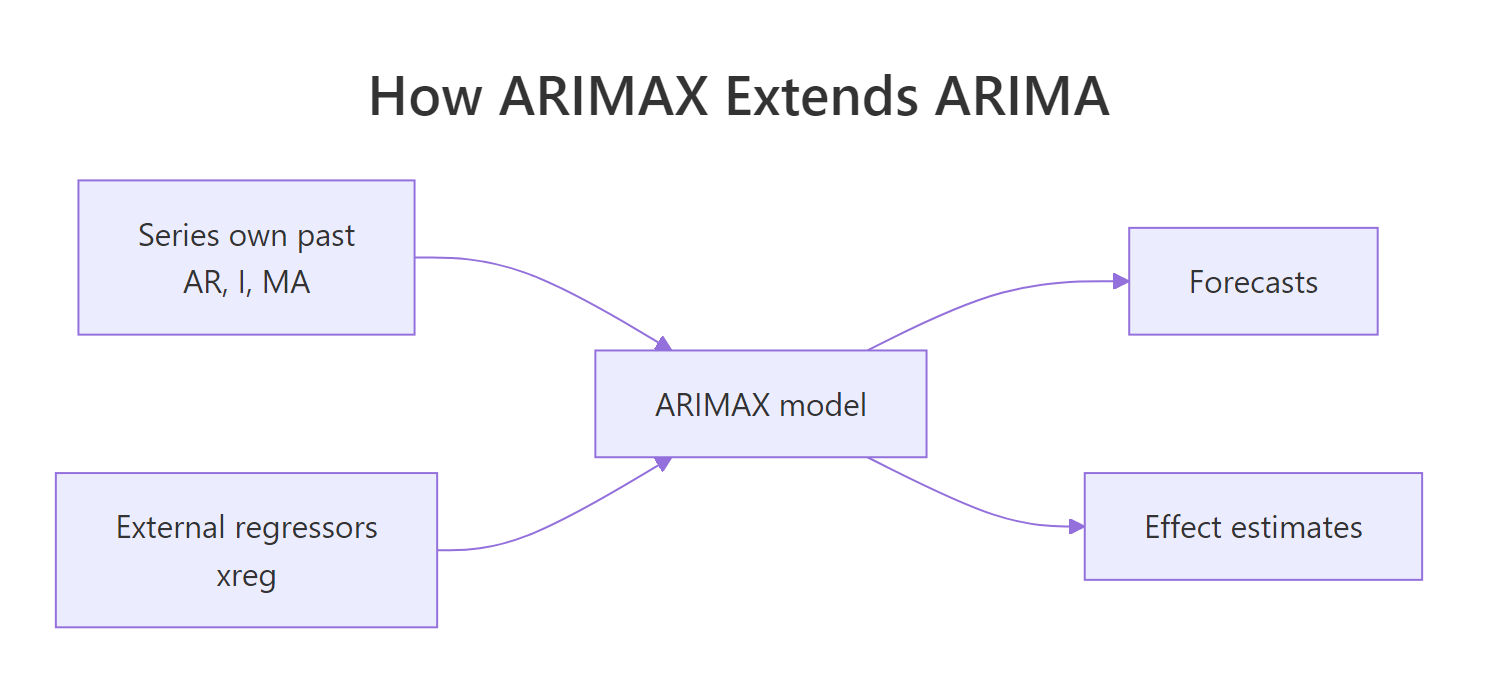
Figure 1: ARIMAX feeds external regressors in alongside a series' own AR, I, and MA structure.
xreg argument just lets the model borrow information from variables outside the series.Try it: Build your own sales series with a temperature effect you choose, then check that ARIMAX recovers it. Change the multiplier below and read the ex_temp coefficient.
Click to reveal solution
Explanation: We built sales with an effect of 5 per degree, and ARIMAX estimated 4.978, off by a hair because of random noise in the sample. Try other multipliers and the coefficient will track them.
How do you fit an ARIMAX model with xreg?
The xreg argument takes a numeric matrix or vector of predictors that lines up with your series row for row. Row 1 of xreg is the value of the regressor at the same time as the first observation of your series (y), and so on. That alignment is the only rule you must respect. When you pass a single predictor, wrapping it in cbind(name = predictor) gives the coefficient a readable name instead of the generic label xreg.
auto.arima() chose the ARIMA orders for us above. You can also fit a specific order by hand with Arima(), which is useful when you want control. Let's fit the same (1, 0, 0) structure manually and confirm we get the identical model.
The output is identical to the automatic fit, which confirms that auto.arima() picked (1, 0, 0) for the error structure. The order = c(1, 0, 0) argument is the familiar c(p, d, q): one AR term, no differencing, no MA term. The xreg sits on top of that, unchanged.
To pull just the temperature effect out of a fitted model, index the coefficient by its name. This is how you would grab the number for a report.
That single number, 3.089, is the practical takeaway of the whole fit: each extra degree of temperature is associated with about 3.09 more sales, after the model has accounted for the day-to-day inertia in the series.
xreg has a different length than y, or has NA values, the fit will fail or mislead. Line the predictor up with the series by date, and fill or drop missing values before fitting.Try it: Fit the model with two AR terms instead of one by changing the order to c(2, 0, 0), then read the temperature coefficient. Does the effect estimate move much?
Click to reveal solution
Explanation: With a second AR term the temperature effect is 3.081, barely different from the 3.089 we saw before. A good regression effect is stable across sensible choices of the error structure, which is a reassuring sign here.
How do you forecast with an ARIMAX model?
Here is the single most important difference between ARIMA and ARIMAX, and the mistake that trips up almost everyone the first time. To forecast ahead, an ARIMAX model needs the FUTURE values of its regressors. It cannot invent them. A plain ARIMA can project itself forward from its own past, but ARIMAX has to be told what temperature will be on each future day before it can forecast sales.
So forecasting is a two-part job: supply the future regressor values, then call forecast(). You pass those future values through the same xreg argument. There is no need to set h (the number of periods): the horizon is simply the number of rows in the future xreg. Let's forecast the next 14 days by giving the model 14 future temperatures.
Each row is one future day. The Point Forecast is the single best guess, and the four interval columns give ranges: the model is 80 percent sure the value lands between Lo 80 and Hi 80, and 95 percent sure between Lo 95 and Hi 95. Look down the point forecasts and you can see them rise and fall, from 106 up to 130 and back down. That wave is the temperature regressor at work: on warmer forecast days the model predicts more sales, exactly as the temperature coefficient says it should.
A picture makes the pattern obvious. The autoplot() function draws the history and the forecast together, with the shaded fan showing the widening uncertainty.
Try it: Forecast just 5 days ahead by building 5 future temperatures. Read the first point forecast.
Click to reveal solution
Explanation: The horizon is 5 because the xreg has 5 rows. The first day's point forecast is about 105.6, and every value reflects the specific future temperature we supplied for that day.
Does the external regressor actually improve the forecast?
Adding a regressor is only worth it if the regressor genuinely helps. The clean way to check is to fit a plain ARIMA on the same series and compare it to the ARIMAX by AICc, the small-sample information criterion where lower is better. Let's fit the plain model first.
Notice the plain model's ar1 is 0.88, much higher than the 0.50 the ARIMAX used. That is telling: without temperature to explain the swings in sales, the AR term has to absorb the temperature-driven movement itself, treating it as if it were inertia. The sigma^2 (the residual variance) is 76.05 here versus 14.5 for the ARIMAX, so the plain model leaves far more unexplained. Now compare the two by AICc.
The ARIMAX AICc of 667 is far below the plain ARIMA's 866. A gap that large is decisive: temperature carries real, useful information about sales, so the model that uses it wins easily. This will not always happen. Some candidate regressors add nothing, and then the plain model scores as well or better. That is exactly why you compare instead of assuming.
Try it: Compute how many AICc points ARIMAX saves over the plain model. Subtract the two values.
Click to reveal solution
Explanation: ARIMAX is 198.95 AICc points better. As a rule of thumb, a difference of more than about 10 is strong evidence for the better model, so this is a landslide in favor of using temperature.
What is R actually fitting when you add xreg?
You may have noticed R never printed the word "ARIMAX." It printed "Regression with ARIMA errors." That wording is not an accident, and understanding it is what separates people who use xreg correctly from people who get confused by it. This short section is the theory; if you only want to use the tool, the practical code above is all you need.
What R fits is a regression, plus a twist. It models your series as a straight-line effect of the regressors, and lets the leftover error follow an ARIMA process instead of being plain independent noise.
$$y_t = \beta_0 + \beta_1 x_t + n_t$$
Where:
- $y_t$ = the observed value at time $t$ (sales today)
- $\beta_0$ = the intercept, the baseline level
- $\beta_1$ = the effect of the regressor, which is the
xregcoefficient - $x_t$ = the external regressor at time $t$ (temperature today)
- $n_t$ = the error term, which itself follows an ARIMA model rather than being pure noise
That last line is the whole point. In an ordinary regression, the errors are assumed to be independent. In time-series data they almost never are: a busy day tends to be followed by another busy day. The ARIMA part of the model exists to soak up that autocorrelation in the errors, so the regression coefficient can be estimated honestly.
To see why this matters, fit a plain regression of sales on temperature and look at its residuals. If the errors were independent, their autocorrelation would be near zero at every lag.
The first value is always 1 (the correlation of the residuals with themselves at lag 0), so ignore it. The next value, 0.494, is the lag-1 autocorrelation, and it is large. Today's regression error is strongly related to yesterday's. That is precisely the structure the ARIMAX picked up as an AR(1) term of 0.50 in the first section. The two numbers, 0.494 from the residuals and 0.50 from the model, are the same fact seen from two angles.
The diagram below sums up the decomposition: the regressors produce a regression effect, the leftover errors are modeled as ARIMA, and the two combine to explain the series.
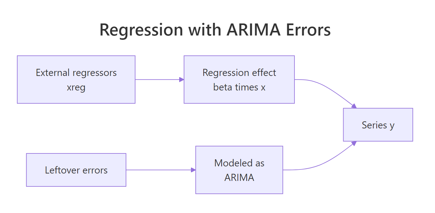
Figure 2: What R fits is a regression on the regressors plus ARIMA-modeled errors.
Arima() and auto.arima() fit, and others mean a different formulation where lagged regressors enter the ARIMA equation directly. This tutorial uses the version R implements, where each coefficient is a clean, contemporaneous effect you can read off and explain.Try it: Read the lag-1 and lag-2 autocorrelations of the regression residuals and connect them to the model's memory.
Click to reveal solution
Explanation: The lag-1 value 0.494 is the strong one, and it fades to 0.168 at lag 2. That decaying pattern is the fingerprint of AR(1) errors, which is exactly the error structure the ARIMAX chose.
Complete Example: Measuring the UK seat belt law
Let's put it together on a famous real dataset and, along the way, meet the second big use of ARIMAX. So far we have used it to forecast. It is just as valuable for measuring the effect of a driver while accounting for the time-series structure around it.
The built-in Seatbelts data records monthly UK road casualties from 1969 to 1984. Britain made front seat belts compulsory on 31 January 1983, and the dataset carries a law column that is 0 before the law and 1 after. We will model the number of drivers killed or seriously injured, using three external regressors: petrol price, distance driven, and the law flag. The law flag is the interesting one: a plain ARIMA could never use it, because it is information from outside the series.
The law column is 0 in these early rows, as expected. We divide kms by 1000 only to keep its coefficient on a readable scale. Now fit a plain seasonal ARIMA and an ARIMAX with the three regressors, and compare them by AICc.
The ARIMAX is better by about 14 AICc points, so the regressors are pulling their weight. Let's look at the full ARIMAX to read the effects.
The seasonal ARIMA orders on the left handle the strong monthly pattern in road casualties, and you can mostly leave them to auto.arima(). The three regressors on the right are what we came for. Focus on law: its coefficient is -279.86, with a standard error of 74.23. Because the coefficient is about 3.8 times its standard error, it is clearly different from zero.
The reading is direct and striking: after accounting for seasonality, petrol price, and how far people drove, the seat belt law is associated with about 280 fewer drivers killed or seriously injured per month. That is the kind of question ARIMAX answers that plain ARIMA cannot even ask. Before trusting any model, though, check its residuals with checkresiduals(), which runs a Ljung-Box test for leftover structure.
Frequently Asked Questions
What is the difference between ARIMA and ARIMAX? ARIMA forecasts a series using only its own past values and errors. ARIMAX adds one or more external predictors through the xreg argument, so the model can also use known drivers like price, weather, or a policy change.
Do I need future values of the regressors to forecast? Yes. This is the key catch. To forecast h steps ahead, you must supply the regressors' values for those future periods via xreg in forecast(). If you do not know them, you either use known scheduled values (like holidays) or forecast the regressors separately first.
Is ARIMAX the same as regression with ARIMA errors? In R's forecast package, yes: Arima() and auto.arima() with xreg fit a regression with ARIMA errors, which R prints by that exact name. The term ARIMAX is used loosely elsewhere and sometimes means a slightly different model, so it helps to know which one you are running.
Can I use a 0/1 dummy variable as a regressor? Absolutely. The seat belt law flag above is a 0/1 dummy, and its coefficient measures the average shift in the series once the flag switches on. Dummies are how you model interventions, promotions, and policy changes.
How many regressors can I use? As many as the data supports, passed as columns of the xreg matrix with cbind(). Just remember every regressor you include for forecasting needs its own future values, and adding predictors that do not help will hurt the model, so compare by AICc.
Practice Exercises
These combine several ideas from the tutorial. Each starter block runs as-is, so write your solution and then reveal ours to compare. The exercises use their own variable names so they will not clash with the code above.
Exercise 1: Recover a known effect from scratch
Build a series my_y that follows a regressor my_x with a true effect of 2.5, plus autocorrelated noise, then fit an ARIMAX and check that it recovers the 2.5. Use set.seed(303).
Click to reveal solution
Explanation: ARIMAX estimated the effect at 2.513, right on top of the true 2.5. It also recovered the baseline near 100 and an AR(1) term near 0.70, matching every value we built into the data.
Exercise 2: Compare a driver's effect across two series
Using the Seatbelts data, fit an ARIMAX to front (front-seat passengers killed or seriously injured) with the same three regressors, compare it to a plain ARIMA by AICc, and read the law coefficient. Is the drop bigger or smaller than the 280 we found for drivers?
Click to reveal solution
Explanation: ARIMAX beats plain ARIMA by about 41 AICc points here, and the law is associated with roughly 202 fewer front-seat casualties per month. It is a large effect, as you would expect, since front-seat passengers were the ones the belt law directly targeted.
Exercise 3: Forecast two temperature scenarios
Using the cafe_fit model from the tutorial, forecast the next 7 days under two scenarios: a heatwave where every day is 32 degrees, and a cold snap where every day is 12 degrees. Compare the first day's point forecast under each. This shows how the future regressor drives the forecast.
Click to reveal solution
Explanation: The heatwave forecast is 141.4 and the cold snap is 79.6, a gap of about 62 sales. That gap is the temperature effect of roughly 3 per degree times the 20-degree difference between the scenarios, which is ARIMAX doing exactly what we taught it.
Summary
ARIMAX is ARIMA with extra input columns. You add known drivers through the xreg argument, and the model separates what the drivers explain from the series' own inertia. The workflow is short and always the same.
| Task | How | Key point |
|---|---|---|
| Add a regressor | xreg = cbind(name = x) |
One column per driver, aligned to y |
| Fit | auto.arima(y, xreg = X) or Arima(y, order, xreg = X) |
auto.arima() picks the error structure |
| Forecast | forecast(fit, xreg = future_X) |
You must supply future regressor values |
| Compare | c(plain$aicc, arimax$aicc) |
Only keep regressors that lower AICc |
| Interpret | coef(fit)["name"] |
The coefficient is a contemporaneous effect |
Keep these takeaways close:
- The X in ARIMAX means external, and it is just one more input column. Everything you know about p, d, and q still applies.
- You must supply future regressor values to forecast. Unlike plain ARIMA, the model cannot project its own inputs.
- Earn every regressor with a comparison. Check AICc with and without it, because useless predictors make forecasts worse.
- What R fits is regression with ARIMA errors. The
xregcoefficient is a clean regression slope, and the ARIMA part gives it trustworthy standard errors. - ARIMAX has two jobs. It sharpens forecasts when you know the drivers, and it measures a driver's effect (like the seat belt law) net of everything else.
References
- Hyndman, R.J., & Athanasopoulos, G. - Forecasting: Principles and Practice, 3rd edition. Chapter 10: Dynamic regression models. Link
- Hyndman, R.J., & Athanasopoulos, G. - Forecasting: Principles and Practice, 2nd edition. Section 9.2: Regression with ARIMA errors in R. Link
- Hyndman, R.J., & Khandakar, Y. - "Automatic Time Series Forecasting: The forecast Package for R." Journal of Statistical Software, 27(3), 2008. Link
- forecast package -
Arima()reference. Link - forecast package -
auto.arima()reference. Link - Nau, R. (Duke University) - Introduction to ARIMA models with regressors. Link
- R Core Team -
Seatbeltsdataset, Road Casualties in Great Britain 1969-84. Link
Continue Learning
- ARIMA in R - the foundation this guide builds on, covering what AR, I, and MA mean and how to fit and forecast one.
- ARIMA Diagnostics in R - go deeper on residual checks and the Ljung-Box test you used to validate the seat belt model.
- SARIMA in R - the seasonal extension that handled the monthly pattern in the road-casualty data.
- ACF and PACF in R - the autocorrelation plots behind the residual checks in this tutorial.