Kalman Filter in R: FKF and KFAS for State Space Models
The Kalman filter is a recursive algorithm that estimates the hidden state of a system from noisy measurements, by repeatedly predicting what comes next and then correcting that prediction with each new observation. This tutorial builds the filter from scratch in base R, proves the hand-coded version reproduces R's built-in filter exactly, then shows the same model in the FKF and KFAS packages.
What problem does the Kalman filter actually solve?
No measurement is exact. A river gauge, a GPS chip and a sales dashboard all report a number that is part real signal and part noise, and you usually care about the signal. R ships with a Kalman filter already installed, so before any theory, watch what it does to a genuinely noisy series: the annual flow of the Nile, measured every year from 1871.
The Nile dataset comes with R, so there is nothing to download. The function StructTS() fits what is called a local level model, which is the simplest possible setup: assume there is a true water level that drifts slowly from year to year, and assume every measurement of it is off by some random amount. StructTS() estimates how big each of those two effects is.
Two numbers came back. level is the estimated variance of the year-to-year drift in the true water level, and epsilon is the estimated variance of the measurement error. Read them as variances, so take square roots to get something interpretable: the true level wanders by about 38 units per year, while any single measurement is off by about 123 units.
That ratio is the whole story. Measurement noise is roughly ten times larger than the real movement, so most of the jaggedness you see in the raw data is not the river changing, it is the gauge being imprecise. Here is what that looks like.
The grey line jumps around violently from year to year. The red line, which is the filter's estimate of the true underlying level, moves smoothly and still captures the one thing that genuinely happened: a sharp drop around 1899, when construction of the first Aswan dam began. The filter kept the real change and threw away the noise.
Notice what the filter did not do. It did not use a moving average, and it did not fit a curve through all the points at once. It walked through the series one year at a time, and at each year it made a guess before seeing the data, then adjusted that guess once the measurement arrived.
Try it: The filtered line is visibly smoother than the raw data. Put a number on that by comparing the standard deviation of the raw Nile series with the standard deviation of the filtered values, which you get from fitted(nile_fit).
Click to reveal solution
Explanation: The raw series varies with a standard deviation of 169.2, the filtered level only 119. The filter removed roughly a third of the variability, and what it removed was the part it judged to be measurement error rather than real change.
What is a state space model, and what is the hidden state?
The Kalman filter does not work on any arbitrary dataset. It works on a specific description of your data called a state space model, and once you can write your problem in that form, the filter follows automatically. So the model comes first.
A state space model says two things. First, there is a quantity you care about that you cannot see directly, called the state. Second, the numbers you actually recorded are that state plus noise. For the Nile, the state is the true average flow of the river in a given year, and the observation is what the gauge printed.
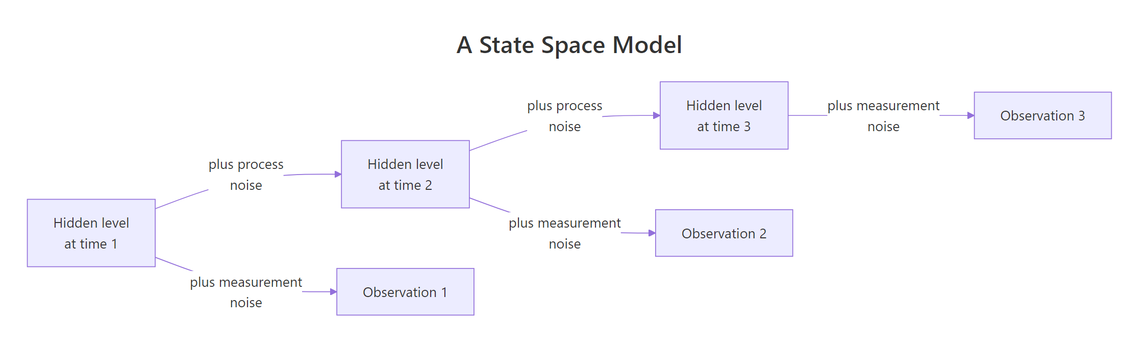
Figure 1: A state space model: a hidden level evolves on its own, and each observation is that level plus measurement noise.
Read the diagram left to right along the top row. The hidden level at time 2 comes from the hidden level at time 1 plus a random nudge. That is the state moving on its own, and nothing you observe influences it. Then read the downward arrows: each observation is the hidden level at that time plus a separate random error.
Those two sentences are the two equations of the model. The observation equation says what you see:
$$y_t = \alpha_t + \varepsilon_t, \qquad \varepsilon_t \sim N(0, \sigma^2_\varepsilon)$$
And the state equation says how the hidden thing moves:
$$\alpha_{t+1} = \alpha_t + \eta_t, \qquad \eta_t \sim N(0, \sigma^2_\eta)$$
Where:
- $y_t$ = the number you actually recorded at time $t$
- $\alpha_t$ = the hidden state at time $t$, the thing you want to know
- $\varepsilon_t$ = measurement error, with variance $\sigma^2_\varepsilon$
- $\eta_t$ = the random nudge that moves the state, with variance $\sigma^2_\eta$
This particular pair of equations is called the local level model, because the state is just a level that wanders. It is the "hello world" of state space modelling, and everything else in this tutorial is a variation on it.
Real data will not tell you whether the filter is doing a good job, because you never get to see the hidden state. So let us build a series where we do know the truth. We will generate a hidden level that wanders with standard deviation 1 per step, then add measurement noise with standard deviation 3 on top of it.
Read the code line by line. cumsum(rnorm(...)) is a random walk: each step adds a fresh random number to the running total, which is exactly the state equation. Adding a second, independent rnorm() on top produces the observation equation. The set.seed(2718) makes every number on this page reproducible on your machine.
Look at the two columns. At time 2 the truth was 9.31 but we recorded 6.02, an error of over 3 units. At time 5 the truth was 8.65 but we recorded 12.07, an error in the other direction. The observations bounce around the truth much more than the truth itself moves.
The blue line is the truth, which in real life you never get to see. The grey dots are your data. Your job, and the filter's job, is to recover the blue line using only the grey dots.
Let us confirm the simulation matches the settings we asked for.
The first line subtracts the truth from the observations to leave pure measurement error. Its standard deviation is 2.99, right on the 3 we specified. The second line takes diff() of the true level to get the step-to-step changes, and their standard deviation is 1.03, matching the 1 we specified.
So measurement noise is about three times larger than the real movement. That ratio is what the filter has to exploit: when noise dominates, trust your prediction more than any single measurement.
Try it: Build a second simulated series where the measurement noise is tiny, standard deviation 0.2 instead of 3, while the hidden level still wanders with standard deviation 1. Store the hidden level in ex_level and the observations in ex_y, then check the size of the measurement error.
Click to reveal solution
Explanation: The measurement error now has a standard deviation of 0.21, far smaller than the level's own movement. In this regime the observations are nearly the truth, so a filter should follow the data closely instead of smoothing it. That is the opposite of the Nile case, and the same algorithm handles both.
How does the Kalman filter combine a prediction with a new observation?
The filter processes one observation at a time, and each observation triggers exactly two moves: a predict step and an update step. Understanding these two moves is understanding the Kalman filter, so we will do them slowly, with real numbers, before writing any loop.

Figure 2: The predict-update cycle that the filter repeats once per observation.
The filter always carries two numbers with it: its current best guess of the level, and how uncertain it is about that guess, expressed as a variance. Call them $a$ and $P$. Everything the filter knows is in those two numbers.
The predict step asks: given what I knew after yesterday, what do I expect today, before looking at today's data? In the local level model the state does not drift in any particular direction, so the best guess for tomorrow's level is today's level. But you become less certain, because the level moved by a random amount you did not observe. So the guess stays put and the uncertainty grows by exactly the size of that random movement.
$$a_{t|t-1} = a_{t-1|t-1}, \qquad P_{t|t-1} = P_{t-1|t-1} + \sigma^2_\eta$$
The notation $t|t-1$ reads "at time $t$, using data up to time $t-1$", so it is the prediction. And $t|t$ reads "at time $t$, using data up to and including time $t$", so it is the updated estimate.
The update step then looks at the actual observation. The gap between what arrived and what you predicted is called the prediction error, or innovation:
$$v_t = y_t - a_{t|t-1}$$
You do not move your estimate by the whole error, because part of that error is just measurement noise. You move by a fraction of it, and that fraction is the Kalman gain:
$$K_t = \frac{P_{t|t-1}}{P_{t|t-1} + \sigma^2_\varepsilon}$$
Where:
- $P_{t|t-1}$ = how uncertain you are about your own prediction
- $\sigma^2_\varepsilon$ = how noisy a single measurement is
- $K_t$ = the resulting weight, always between 0 and 1
Look at that fraction rather than memorising it. The numerator is your own uncertainty, the denominator is your uncertainty plus the measurement's uncertainty. So the gain is the share of the total uncertainty that belongs to you. If you are very unsure and the instrument is precise, the gain approaches 1 and you jump nearly all the way to the new measurement. If you are confident and the instrument is noisy, the gain approaches 0 and you barely move.
The estimate and its uncertainty then update:
$$a_{t|t} = a_{t|t-1} + K_t v_t, \qquad P_{t|t} = (1 - K_t) P_{t|t-1}$$
That second equation is worth a second look: uncertainty always shrinks in the update, because $K_t$ is between 0 and 1. Every observation, no matter how noisy, tells you something.
If you would rather skip the algebra, the code below does exactly what these four lines say, and reading it is enough.
Let us run the very first step by hand. The filter has to start somewhere, so we start it at the first observation, 9.15, and declare that we are extremely unsure about it by setting the variance to 100. That large number is a way of saying "I know essentially nothing yet".
The gain came out at 0.917, very close to 1, because our starting uncertainty of 100 is more than ten times the measurement variance of 9. A gain that high means the filter moves almost all the way to the measurement, and since we deliberately started it at that same measurement, the level has nowhere to move and stays at 9.155. The number that really changed here is the variance, which collapses from 100 down to 8.257. One observation bought us a lot of confidence.
Now predict forward to time 2. The level guess stays where it is, and the variance grows by the state noise variance, which is $1^2 = 1$.
The prediction for time 2 is still 9.155, but the uncertainty has crept up from 8.257 to 9.257. That growth is the price of time passing: the river moved and we did not watch it.
Now the second observation arrives, and we update again.
Three numbers, and each one is meaningful. The prediction error is -3.133, meaning the observation of 6.02 came in far below the predicted 9.155. The gain has dropped from 0.917 to 0.507, because the filter is no longer clueless. And so the estimate moves by only about half the error, landing at 7.566 rather than following the data all the way down to 6.02.
That halfway move is the whole point of the gain: some of that -3.133 gap is the hidden level genuinely falling, and some of it is measurement noise, so the error is split between the two in proportion to the two variances.
Try it: Suppose the filter has been running a long time and is now very confident, with a predicted variance of only 0.5, while the measurement variance is still 9. Compute the Kalman gain and store the variance in ex_P.
Click to reveal solution
Explanation: The gain is 0.053, so the filter moves only about 5% of the way toward each new observation and ignores the other 95%. A confident filter with a noisy instrument becomes very hard to push around, which is exactly what you want when the data are unreliable.
How do you code a Kalman filter from scratch in R?
You have now done every operation the filter performs. Turning it into a loop is mechanical: repeat predict and update for every observation, carrying $a$ and $P$ forward each time.
The function below takes the observed series, the two noise standard deviations, and starting values for the estimate and its variance. It returns the filtered level at every time point, the variance at every time point, and the gain at every time point, because watching the gain evolve is genuinely instructive.
Three lines inside the loop are the update step, in the same order you just did by hand: gain, then estimate, then variance. The two lines after them are the predict step for the next iteration, and in the local level model the level prediction is simply the current estimate, which is why a_pred <- level[t] looks so plain.
That is the entire Kalman filter for this model. Twelve lines, no packages. Let us run it on the simulated data using the true noise values we generated with.
Check row 2 against the hand calculation: the filtered value is 7.57, matching the 7.566 we computed manually. The loop is doing exactly what we did by hand.
Now compare columns. At time 5 the observation spiked to 12.07 while the truth was 8.65, and the filter moved only to 9.01. The observation jumped 4.28 units from the previous one and the filtered level moved 1.34, so most of the spike was left out. Holding that much back is the entire value of the method, and we can measure it.
Root mean squared error against the known truth fell from 2.98 to 1.6. The filter cut the typical error nearly in half, using nothing but the two variance settings and the order of the data. This is the comparison you can never make on real data, which is exactly why we simulated.
Now watch the gain, which is where the filter's changing confidence shows up.
The gain starts at 0.917, drops fast over the first few observations, and then settles at 0.282 and stays there. That settled value is called the steady state gain, and it depends only on the ratio of the two variances, not on the data.
The curve falls steeply then flattens. After roughly ten observations the filter has learned as much about its own precision as it ever will, and from then on it applies a fixed 28% correction to every prediction error.
Try it: Rerun kalman_1d() on y_obs with a much noisier instrument, sigma_meas = 10 instead of 3, keeping everything else the same. Store the result in ex_kf and report the final gain. Predict whether it will be higher or lower than 0.282 before you run it.
Click to reveal solution
Explanation: The settled gain drops from 0.282 to 0.095. Telling the filter the instrument is three times noisier makes each correction about a third as large, so it now moves less than a tenth of the way toward each new reading. The data never changed, only our stated belief about the data.
How do you run the Kalman filter with base R's StructTS?
So far we cheated: we told the filter the true noise variances because we generated the data. On real data you do not know them, so they have to be estimated from the series itself, by maximum likelihood. Maximum likelihood here means trying candidate pairs of variances, asking of each pair how probable the series you actually recorded would be if that pair were correct, and keeping the pair that makes it most probable.
You do not need a package for this. Base R's StructTS() fits the local level model and estimates both variances at once. Let us point it at the simulated series and see whether it can recover the settings we know are correct: a state variance of $1^2 = 1$ and a measurement variance of $3^2 = 9$.
It recovered 0.995 against a true value of 1, and 8.647 against a true value of 9. From 100 noisy observations and no other information, maximum likelihood untangled the two variances almost exactly. That is the part beginners usually find hard to believe, which is why it is worth checking against a known truth.
Now the important verification. If our hand-coded filter is really the Kalman filter, then feeding it these estimated variances should reproduce StructTS()'s own output. Note the wider initial variance of 1e7, which matches how StructTS() initialises.
Identical to four decimal places. Let us push it further and take the largest disagreement across all 100 time points.
The biggest gap anywhere in the series is 0.0000142, which is rounding error from the printed coefficients we fed in. Your twelve-line function and R's compiled implementation are the same algorithm.
There is one more distinction to nail down, because it trips people up constantly. Everything so far is filtering: the estimate at time $t$ uses only data up to time $t$. That is what you want in real time, when the future has not happened yet. But if you have the whole series in hand already, you can do better at every point by also using later observations. That is called smoothing, and base R gives it to you with tsSmooth().
Look at row 3. The observation was 963, a big dip. The filtered estimate fell to 1072.8, because at that moment the filter did not know what came next. The smoothed estimate barely moved, staying at 1105.3, because it can see that 1210 arrived immediately afterwards and concludes the 963 was mostly measurement noise.
The smoothed column is visibly steadier across all five rows. Hindsight is genuinely worth something.
Try it: The Nile model assumed the level only wanders with no persistent direction. Fit the richer version that also allows a slope, using StructTS(Nile, type = "trend"), store it in ex_trend, and look at the estimated variances.
Click to reveal solution
Explanation: The slope variance is estimated as 0.0, so maximum likelihood concluded the Nile has no persistent trend component at all and set it to zero. The level and epsilon variances barely changed from the simpler model. This is a useful diagnostic: fitting a component and getting a zero variance back is the model telling you that component is not needed.
How do you use the FKF package for fast Kalman filtering?
Base R's StructTS() is convenient but rigid. It offers three fixed model shapes, one series at a time, and no way to express anything unusual. When you need full control, you write the state space model as matrices yourself, and the FKF package (Fast Kalman Filter) is the leanest way to do that in R.
FKF gives you one main function, fkf(), implemented in C. It handles multiple series at once, allows every parameter to change over time, and is the fastest general option in R. The cost is that you must supply the model as raw matrices, which is where most people get stuck. So here is the complete map.
The general state space model FKF implements is:
$$\alpha_{t+1} = d_t + T_t \alpha_t + \eta_t, \qquad y_t = c_t + Z_t \alpha_t + \varepsilon_t$$
Every argument of fkf() corresponds to one piece of those two equations.
| Argument | Role in the model | Shape required |
|---|---|---|
a0 |
Starting value of the state | vector, length m |
P0 |
Starting variance of the state | matrix, m x m |
dt |
Constant added in the state equation | matrix, m x 1 |
ct |
Constant added in the observation equation | matrix, d x 1 |
Tt |
How the state moves to the next step | array, m x m x 1 |
Zt |
How the state maps into observations | array, d x m x 1 |
HHt |
Variance of the state noise | array, m x m x 1 |
GGt |
Variance of the measurement noise | array, d x d x 1 |
yt |
Your data | matrix, d x n |
Here m is the number of hidden states and d is the number of observed series. For our local level model both are 1, so every matrix is 1 x 1. The final dimension of the arrays is the time dimension: use 1 when a parameter is constant, or n when it changes every period.
The single most common error is the data layout, so start there.
library(FKF)
y_nile <- rbind(as.numeric(Nile))
dim(y_nile)
#> [1]   1 100
rbind() produces a 1 x 100 matrix: one row because there is one series, 100 columns because there are 100 time points. Series go in rows and time goes across columns, which is the transpose of how most R users instinctively lay out data.
Now the filter itself. We already know from StructTS() that the Nile's variances are about 1469 and 15099, so we can plug them straight in and confirm FKF agrees.
fkf_nile <- fkf(a0  = y_nile[1, 1],
                P0  = matrix(1e7),
                dt  = matrix(0),
                ct  = matrix(0),
                Tt  = array(1, c(1, 1, 1)),
                Zt  = array(1, c(1, 1, 1)),
                HHt = array(1469, c(1, 1, 1)),
                GGt = array(15099, c(1, 1, 1)),
                yt  = y_nile)
round(fkf_nile$logLik, 2)
#> [1] -641.52
round(fkf_nile$att[1, 1:5], 1)
#> [1] 1120.0 1140.9 1072.8 1117.3 1130.0
Every argument here is the local level model written out. Tt = 1 says the next level equals the current level, Zt = 1 says the observation reads the level directly, dt and ct are zero because nothing is added, and P0 = 1e7 is the diffuse start.
Now compare fkf_nile$att with the filtered column that fitted(nile_fit) gave us in the base R section: 1120.0, 1140.9, 1072.8, 1117.3, 1130.0, identical. Two completely different implementations, same numbers.
The logLik element is what makes parameter estimation possible: run the filter with candidate variances, read off the log-likelihood, and let an optimiser search for the best pair. That is precisely what StructTS() does internally, and we can reproduce it.
nile_negll <- function(par) {
  -fkf(a0 = y_nile[1, 1], P0 = matrix(1e7), dt = matrix(0), ct = matrix(0),
       Tt = array(1, c(1, 1, 1)), Zt = array(1, c(1, 1, 1)),
       HHt = array(exp(par[1]), c(1, 1, 1)),
       GGt = array(exp(par[2]), c(1, 1, 1)),
       yt = y_nile)$logLik
}
mle <- optim(c(log(1000), log(15000)), nile_negll, method = "BFGS")
round(exp(mle$par))
#> [1]  1469 15099
Two details make this work. The function returns the negative log-likelihood because optim() minimises. And the parameters are optimised on the log scale, then exponentiated inside, which guarantees the variances stay positive no matter where the optimiser wanders.
The answer is 1469 and 15099, matching StructTS()'s 1469.1 and 15098.6. You have now estimated a state space model from raw matrices and reproduced base R's result.
Finally, FKF's smoother takes the filter output directly.
fkf_smooth <- fks(fkf_nile)
round(fkf_smooth$ahatt[1, 1:5], 1)
#> [1] 1111.7 1110.9 1105.3 1113.5 1112.4
These are the same smoothed values tsSmooth() produced: 1111.7, 1110.9, 1105.3, 1113.5, 1112.4. Note that fks() takes the fitted filter object rather than the data, because smoothing is a backward pass over results the filter already computed.
Try it: The local linear trend model has two states, level and slope, where the next level is level plus slope. Its transition matrix is therefore matrix(c(1, 0, 1, 1), nrow = 2) and its observation matrix picks out only the level. Build both as ex_Tt and ex_Zt, then multiply ex_Zt %*% ex_Tt to see what the observation equation reads after one step.
Click to reveal solution
Explanation: ex_Tt has a 1 in the top-right corner, which is what adds the slope into the level at each step. ex_Zt is [1, 0], so observations see the level and never the slope directly. Their product [1, 1] shows that after one step forward, the observation depends on both the old level and the old slope, which is how a trend gets into the data even though it is never measured.
How do you build state space models with KFAS?
FKF is fast but verbose, and writing matrices by hand gets painful the moment you want a trend plus a seasonal pattern. KFAS solves that with a formula interface: you describe the model in components, and it assembles the matrices for you.
The pattern has three steps. SSModel() defines the model, fitSSM() estimates any unknown variances, and KFS() runs the filter and smoother. Anywhere you write NA in the model definition, you are saying "estimate this from the data".
library(KFAS)
nile_model <- SSModel(Nile ~ SSMtrend(degree = 1, Q = list(NA)), H = NA)
nile_mle   <- fitSSM(nile_model, inits = c(log(1000), log(15000)), method = "BFGS")
round(c(Q = nile_mle$model$Q[1, 1, 1], H = nile_mle$model$H[1, 1, 1]))
#>     Q     H
#>  1469 15099
Read the formula. SSMtrend(degree = 1) is the local level component, where degree 1 means level only and degree 2 would add a slope. Q is the state noise variance and H is the measurement noise variance, both set to NA so fitSSM() estimates them.
The answer is 1469 and 15099 again. That is now three independent routes to the same pair of numbers.
Running KFS() gives you filtering and smoothing in one object. The filtered states live in att and the smoothed states in alphahat.
kfas_out <- KFS(nile_mle$model)
round(data.frame(filtered = kfas_out$att[1:5], smoothed = kfas_out$alphahat[1:5]), 1)
#>   filtered smoothed
#> 1   1120.0   1111.7
#> 2   1140.9   1110.9
#> 3   1072.8   1105.3
#> 4   1117.3   1113.5
#> 5   1130.0   1112.4
Both columns match what base R and FKF produced. The naming is worth memorising because it is easy to grab the wrong one: att is filtered and uses only the past, alphahat is smoothed and uses the whole series.
KFAS also gives you uncertainty around the estimate, which the earlier tools made you compute yourself.
nile_band <- predict(nile_mle$model, interval = "confidence", level = 0.95)
round(head(nile_band, 4), 1)
#> Time Series:
#> Start = 1871
#> End = 1874
#> Frequency = 1
#>         fit    lwr    upr
#> 1871 1111.7  987.2 1236.1
#> 1872 1110.9  999.2 1222.5
#> 1873 1105.3 1001.2 1209.3
#> 1874 1113.5 1013.7 1213.3
In 1871 the estimated level is 1111.7 with a 95% interval from 987.2 to 1236.1. That band is narrower in later years because the smoother has observations on both sides, whereas 1871 only has the future to lean on.
KFAS goes considerably further than the local level model. SSMseasonal() adds seasonal components, SSMregression() adds explanatory variables with possibly time-varying coefficients, SSMarima() embeds an ARIMA structure, and the distribution argument handles Poisson, binomial, negative binomial and gamma observations, which no other option here supports.
Try it: The ratio of state variance to measurement variance decides how much smoothing you get, and it is called the signal-to-noise ratio. Compute it for the Nile from nile_fit$coef, which you fitted in the first section, and store it in ex_ratio.
Click to reveal solution
Explanation: The ratio is 0.0973, so the real signal carries under a tenth of the variance of the measurement error. A small ratio means heavy smoothing, which is exactly what the flat red line in the first plot showed. If this number were above 1, the filter would track the data closely instead.
How do you handle missing data and forecast ahead?
Missing observations wreck most time series methods. In a state space model they need no special handling at all, and understanding why is the moment the whole framework clicks.
Each time step does two things: predict, then update using the observation. If there is no observation, you simply skip the update. The state carries forward on its prediction alone, and because the predict step always adds state noise to the variance, your uncertainty grows a little each period until real data returns.
You can see this in our own function. Here it is with one if added.
The whole change is the if (is.na(y[t])) branch, which copies the prediction straight into the output and leaves the variance alone. Everything else is untouched.
Read the two columns. The level freezes at 12.69 the moment data stops, because with nothing to correct against, the best guess never changes. But the standard deviation climbs steadily from 1.59 to 2.56, because every missing step adds the state noise variance and no observation arrives to take any back.
Let us watch the uncertainty across the whole gap and past its end.
Uncertainty more than doubles across the gap, from 1.59 to 3.68, then collapses back to 2.36 the instant a real observation arrives at time 51. One measurement recovered most of eleven periods of lost confidence.
KFAS applies this automatically. Below we blank out twenty years of the Nile and let the smoother fill them in, reusing the variances estimated earlier.
nile_hole <- Nile
nile_hole[21:40] <- NA
hole_model <- SSModel(nile_hole ~ SSMtrend(degree = 1, Q = list(nile_mle$model$Q[1, 1, 1])),
                      H = nile_mle$model$H[1, 1, 1])
hole_out <- KFS(hole_model)
round(hole_out$alphahat[c(19, 21, 30, 40, 41)], 1)
#> [1] 995.7 990.1 903.4 807.2 797.5
We passed the fitted variances as fixed numbers instead of NA this time, since we already estimated them. Inside the hole the smoother does not hold a constant: it slides from 990.1 at year 21 down to 807.2 at year 40, interpolating smoothly between the last value before the gap and the first value after it. The filter alone would have held flat, but the smoother sees both sides.
Forecasting uses the same predict() call with n.ahead.
nile_fc <- predict(nile_mle$model, n.ahead = 5, interval = "prediction", level = 0.95)
round(nile_fc, 1)
#> Time Series:
#> Start = 1971
#> End = 1975
#> Frequency = 1
#>        fit   lwr    upr
#> 1971 798.4 517.1 1079.7
#> 1972 798.4 507.2 1089.5
#> 1973 798.4 497.7 1099.1
#> 1974 798.4 488.4 1108.3
#> 1975 798.4 479.4 1117.3
The point forecast is flat at 798.4 for all five years, which is correct: a local level model has no trend, so its best guess for every future year is the current level. What changes is the interval, widening from 562 units across in 1971 to 638 in 1975. The point forecast does not get worse further out, the band around it just gets wider, because each extra year with no observation adds another dose of state variance.
Finally, something a local level model cannot do. AirPassengers has both a rising trend and a strong yearly cycle, so we need a trend component and a seasonal component together. Working in logs stabilises the growing seasonal swings.
air_log <- log10(AirPassengers)
air_model <- SSModel(air_log ~ SSMtrend(degree = 2, Q = list(NA, NA)) +
                       SSMseasonal(period = 12, sea.type = "dummy", Q = NA), H = NA)
air_mle <- fitSSM(air_model, inits = rep(-5, 4), method = "BFGS")
air_out <- KFS(air_mle$model)
round(coef(air_out)[144, 1:3], 4)
#>      level      slope sea_dummy1
#>     2.6843     0.0041    -0.0478
Three components, added with + exactly like lm(). degree = 2 gives level and slope, and SSMseasonal(period = 12) gives a monthly pattern. Four variances are estimated here, hence four starting values in inits.
The final row decomposes the last month of data. The level sits at 2.6843 on the log10 scale, which is about 483 passengers. The slope is 0.0041 per month, meaning the trend is still climbing by roughly 1% a month. And the seasonal term is -0.0478, so December runs about 10% below the trend line.
air_fc <- predict(air_mle$model, n.ahead = 6, interval = "prediction", level = 0.95)
round(10^air_fc)
#>          fit lwr upr
#> Jan 1961 457 423 494
#> Feb 1961 438 400 481
#> Mar 1961 490 441 545
#> Apr 1961 501 445 564
#> May 1961 505 443 576
#> Jun 1961 568 493 655
Because we modelled log10(AirPassengers), we raise 10 to the power of the forecast to get passengers back. The forecast dips in February and climbs into June, reproducing the real seasonal shape, and the intervals widen from 71 passengers across in January to 162 in June.
Try it: In kalman_na() the uncertainty grows during a gap at a rate set by sigma_proc. Rerun the gap filter with sigma_proc = 4 instead of 1, store it in ex_gap, and report the standard deviation at time 50, the last missing point. Compare it to the 3.68 we got before.
Click to reveal solution
Explanation: The standard deviation at the end of the gap rises from 3.68 to 13.51, nearly four times higher. Telling the filter the level can move by 4 units per step means each unobserved step adds sixteen times the variance it added before, and eleven of them accumulate. How fast you believe the state moves directly controls how fast your uncertainty grows once the data stops.
When should you choose base R, FKF, or KFAS?
All three fit the same models and return the same numbers, so the choice is about interface, speed and how unusual your model is.
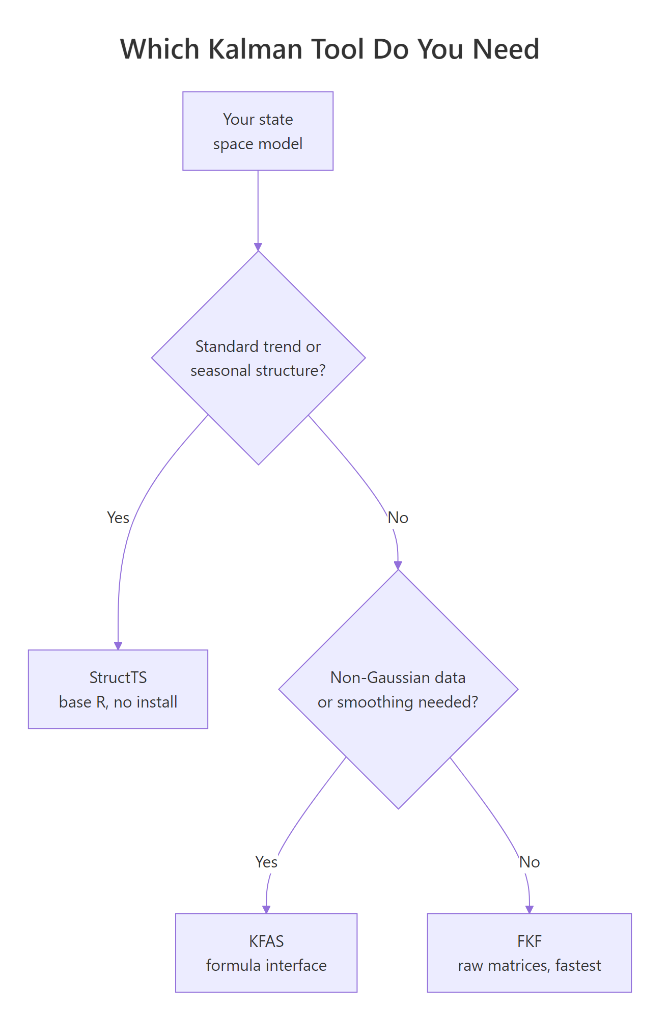
Figure 3: Choosing between StructTS, FKF and KFAS.
| Capability | StructTS (base R) | FKF | KFAS |
|---|---|---|---|
| Installation | none needed | CRAN | CRAN |
| How you specify the model | three fixed types | raw matrices | formula components |
| Speed | adequate | fastest | fast |
| Smoothing | tsSmooth() |
fks() |
built into KFS() |
| Non-Gaussian observations | no | no | yes |
| Time-varying parameters | no | yes | yes |
| Multiple series at once | no | yes | yes |
| Learning curve | lowest | steepest | moderate |
The practical rule follows the diagram. If your model is a level, a trend, or a basic structural model with seasonality, StructTS() needs no install and no matrices. If you need count or binary observations, or you want trend plus seasonal plus regressors written readably, use KFAS. If you are running a custom model thousands of times inside an optimiser or a simulation, FKF's raw matrix interface is the fastest thing available.
One honest caveat: none of these do nonlinear models. If your state equation is not linear, you need an extended or unscented Kalman filter, or else a particle filter. Those live in other packages entirely.
Try it: Confirm the link between the signal-to-noise ratio and the steady state gain on the simulated series. Compute the ratio from sim_fit$coef into ex_sn, then print the last value of kf$gain and see whether a ratio near 0.1 goes with a gain near 0.28.
Click to reveal solution
Explanation: A signal-to-noise ratio of 0.115 produces a steady state gain of 0.282. The gain is always larger than the ratio, because the filter accumulates information over many periods rather than judging each observation on its own. Note too that the Nile's ratio of 0.0973 is close to this series' 0.115, which is why both got heavily smoothed.
Practice Exercises
These combine several ideas from the tutorial. Each uses fresh variable names so nothing above gets overwritten.
Exercise 1: Filter a very quiet signal buried in loud noise
Simulate 200 observations where the hidden level wanders with standard deviation 0.5 around a start of 50, and measurement noise has standard deviation 4. Use set.seed(1848), and generate the level before the noise. Filter it with kalman_1d() using the true noise values and a diffuse start, then report the RMSE of the raw observations and of the filtered level against the truth. Name your objects cap_level, cap_y and cap_kf.
Click to reveal solution
Explanation: The error drops from 3.69 to 1.13, a threefold improvement, much better than the halving we saw earlier. The signal-to-noise ratio here is 0.5^2 / 4^2, about 0.016, far smaller than before. The noisier the measurements relative to the real movement, the more a Kalman filter buys you.
Exercise 2: Extract one-step-ahead forecasts and check them
The filter's prediction error y[t] - a_pred is a genuine one-step-ahead forecast error, called an innovation. If the model is correct, innovations should average about zero and show no autocorrelation, because any predictable pattern left in them is information the filter failed to use.
Write kalman_forecast(), a variant of kalman_1d() that also records the prediction a_pred before each update, and returns onestep, level and error. Run it on y_obs with the true noise values, report the mean and standard deviation of the errors, then check the first three autocorrelations with acf(..., plot = FALSE).
Click to reveal solution
Explanation: The mean error is -0.417, close to zero relative to a standard deviation of 3.462, and all three autocorrelations sit between -0.113 and 0.169, well inside the rough 95% band of 1.96/sqrt(100) = 0.196. The innovations look like noise, so the model has extracted what was extractable. This is the standard diagnostic for a fitted state space model.
Exercise 3: Decompose AirPassengers with a basic structural model
StructTS() has a third type, "BSM", the basic structural model, which fits level, slope and seasonal components at once. Fit it to log10(AirPassengers), store it in cap_struct, and print the four estimated variances rounded to six decimal places. Then decide which component carries the real movement and which are effectively switched off.
Click to reveal solution
Explanation: Two variances came back as zero. A zero epsilon says the model found no measurement noise at all, so it treats every observation as exact and the components absorb all the movement. A zero slope variance means the trend's direction is fixed rather than wandering. The action is in seas at 0.000263 and level at 0.000146, so the seasonal pattern actually moves around more from year to year than the underlying level does, which matches the widening yearly swings visible in the raw series.
FAQ
Is the Kalman filter only for time series?
No. It applies to anything where a hidden quantity evolves in steps and you get noisy readings of it, which is why it appears in GPS navigation, robotics and sensor fusion as often as in economics. The requirement is the model shape, a state equation plus an observation equation, not the fact that the index happens to be time.
What is the difference between the Kalman filter and a moving average?
A moving average applies fixed weights to a fixed window regardless of the data. The Kalman filter derives its weight, the gain, from your stated noise variances and updates its own uncertainty as it goes, so it smooths hard when measurements are unreliable and tracks closely when they are precise. It also gives you a variance at every point, which a moving average never does.
Do I need to know the noise variances in advance?
No. Estimate them from the data by maximum likelihood, which is what StructTS() does automatically and what the optim() example with FKF does explicitly. You only need starting values, and the log scale trick shown above keeps them positive during the search.
Why did my fitted variance come back as exactly zero?
That is the model telling you the component is not needed, as happened with the slope on the Nile and with epsilon in Exercise 3. It is a legitimate answer at the boundary of the parameter space, not an error, though it does mean standard errors for that component are not trustworthy.
Should I use the filtered or the smoothed estimate?
Use filtered values for anything that must run in real time, because they use only past data. Use smoothed values for historical analysis and decomposition, where the whole series is already available. Reporting smoothed values as if they were live estimates is the most common serious mistake with these models.
Can the Kalman filter handle nonlinear models?
Not the standard one, which assumes both equations are linear with Gaussian noise. Nonlinear problems need an extended or unscented Kalman filter, or a particle filter, and those live in other packages. KFAS does relax the Gaussian assumption on the observations, supporting Poisson, binomial, negative binomial and gamma data.
Why does FKF want three-dimensional arrays for constant parameters?
Because the last dimension is time, and FKF allows every parameter to change at every step. Passing array(1, c(1, 1, 1)) means "one state, one series, constant across time", while passing a length-n final dimension lets the parameter vary. The uniform shape is what makes time-varying models possible without a separate interface.
Summary
| Idea | What to remember |
|---|---|
| State space model | Two equations: a hidden state that evolves, and observations that are the state plus noise |
| Local level model | The simplest one, a random-walk level observed with error, fitted by StructTS(type = "level") |
| Predict step | Carry the state forward and let its variance grow by the state noise |
| Update step | Move toward the new observation by the Kalman gain times the prediction error |
| Kalman gain | Your uncertainty divided by total uncertainty, between 0 and 1, settling to a constant |
| Signal-to-noise ratio | State variance over measurement variance; small means heavy smoothing |
| Filtering vs smoothing | Filtered uses only the past and is safe for live use; smoothed uses the whole series |
| Missing data | Skip the update, keep the prediction, let the variance grow |
| Forecasting | Filtering forward with all future observations treated as missing |
| StructTS | Base R, no install, three fixed model types |
| FKF | Raw matrices, fastest, time-varying parameters, series in rows |
| KFAS | Formula interface, seasonal and regression components, non-Gaussian observations |
The single most useful takeaway is that these are all one algorithm. Once you can write your problem as a state equation and an observation equation, filtering, smoothing, interpolation and forecasting all fall out of the same recursion, and the package you use is a matter of convenience.
References
- Helske, J. (2017). KFAS: Exponential Family State Space Models in R. Journal of Statistical Software, 78(10), 1-39. The paper behind KFAS, and the clearest write-up of the general state space model it implements. Link
- KFAS package on CRAN: reference manual and vignettes, including worked
SSMtrendandSSMseasonalexamples. Link - FKF package on CRAN: the Fast Kalman Filter reference manual, with the exact required shape of every matrix argument. Link
- R Core Team: the
StructTShelp page, for the three model types base R fits and what its coefficients mean. Link - R Core Team: the
KalmanLikehelp page, documenting the Kalman filter functions underneathStructTSandarima. Link - R Core Team: the
tsSmoothhelp page, on fixed-interval smoothing of structural models. Link - Petris, G., Petrone, S. and Campagnoli, P. dlm: an R package for Bayesian analysis of Dynamic Linear Models. Package vignette, and the route to take if you want the Bayesian treatment of the same models. Link
- R Core Team: the
Niledataset documentation, describing the flow measurements from 1871 to 1970 used throughout this tutorial. Link
Continue Learning
- ARIMA in R: the other classical route to modelling a time series, and R's
arima()uses a Kalman filter internally to compute its likelihood. - ETS Models in R: exponential smoothing, whose simplest form is mathematically equivalent to the local level model you filtered here.
- Time Series Decomposition in R: splitting a series into trend, seasonal and remainder, the same job the basic structural model did in Exercise 3.