Conformal Prediction in R: Distribution-Free Forecast Intervals
Conformal prediction builds a forecast interval out of the mistakes your model has already made. You let the model forecast data it never trained on, collect how far off it was, take a quantile of those errors, and use that number as your interval width. No bell curve, no assumption that the model is correctly specified, and it wraps around any forecasting method you like, including ones that have no interval theory at all. This page builds it from scratch in base R and the forecast package, then audits it against a real series where the textbook intervals are measurably wrong. Every number below was produced by running the code, not estimated.
Does a 95% prediction interval really contain the truth 95% of the time?
A prediction interval makes a specific, checkable promise: over many forecasts, the truth should land inside the interval 95% of the time. Almost nobody checks. We are going to check first and build second, because the size of the gap is what motivates everything else on this page.
The series is Australian monthly wine sales, which ships with the forecast package. It runs from January 1980 to August 1994 and it has the two properties that make forecasting interesting: a strong December spike every year, and a slow drift upward in overall volume.
176 monthly observations, twelve per year. Let us look at it before we model it.
You can see the annual sawtooth and the upward drift. Now we fit a model. ets() picks an exponential smoothing model automatically, which means it works out for itself whether the trend and the seasonal pattern should be added on or multiplied in. It is a strong, standard choice for a series shaped like this one, and it hands back a prediction interval for free.
That is a normal, respectable forecast. September 1994 sales will be about 24,739 bottles, and the model is 95% confident the truth lies between 20,464 and 29,013.
Here is the walk-through. ets(sales) estimated the smoothing model, forecast() projected it six months forward, and level = 95 asked for bounds wide enough to hold the truth 95% of the time. The interpretation is that if you plan on this, you should be surprised by an outcome outside those bounds roughly one month in twenty.
Should you be? We can find out, because we have fourteen years of history. The idea is simple: pretend we are standing at some point in the past, make a one-month-ahead forecast with a 95% interval, then step forward and see whether the real value landed inside. Do that at every possible point in the series and count.
Read the loop from the inside out. subset(sales, end = i) gives the model only the history available at time i, so nothing from the future leaks in. ets(..., model = base) reuses the smoothing parameters we estimated once at the start and simply feeds them the new observations, and use.initial.values = TRUE keeps that first fit's starting level and seasonal figures too, so nothing at all is re-estimated inside the loop. forecast(..., h = 1) steps one month ahead, and the last line marks whether the real value fell between the bounds.
The first four forecasts all landed inside, which is what you want to see. The question is what happens across all 128 of them.
subset(sales, end = i), which hands the model history up to month i and nothing beyond. It is easy to lose that guard by scaling or differencing the full series before the loop, or by fitting on everything and then slicing predictions afterwards. Both mistakes make coverage look excellent and both are silent.The model made 128 one-month-ahead forecasts and its 95% interval held the truth 108 times. That is 84.4%, not 95%. Instead of being blindsided once every twenty months, you would have been blindsided once every six and a half.
Nothing here is a trick. ets() chose its own model form, it saw only past data at every step, and the series is a well-behaved commercial time series with no crashes or missing values. The interval is simply narrower than reality.
level = 95 describes what the model's assumptions imply, not what the model achieved. Until you roll the model forward over held-out data and count, you have a label rather than a fact, and on this series the label was wrong by more than ten percentage points.Try it: Rerun the audit at level = 80 instead of 95 and report the coverage you actually get. Reuse base and origins so you are not refitting anything new.
Click to reveal solution
Explanation: The 80% interval covers 60.2% of the time. Narrowing the interval did not just shrink coverage proportionally, it made the shortfall worse in relative terms, because the parametric bounds get their shape from the same distributional assumption at every level.
What is a conformal prediction interval?
The parametric interval failed because it was derived rather than measured. ets() estimates one number for the size of a typical error, assumes errors follow a bell curve, and multiplies. If either half of that is wrong, the interval is wrong.
Conformal prediction throws the derivation away and measures instead. Its whole premise fits in one sentence: the mistakes the model has already made are the best available forecast of the mistake it is about to make. So you gather those mistakes and read the answer off them directly.
Let us see why the derived interval was too narrow. We can compare the width a bell curve implies against the errors that actually occurred.
The walk-through: audit$err is how far the truth was from the point forecast each month, sd() measures their typical spread, and 1.96 * sd is the textbook half-width of a 95% Gaussian interval. The last two lines ask the data directly how big the errors really got.
The interpretation is that the bell curve says 95% of errors should be within 6,230 bottles, but the real 95th percentile is 6,593, and the worst month was off by 9,380. The tails are fatter than a normal distribution allows. That is not unusual, it is the ordinary condition of real data, and it is exactly the assumption conformal prediction refuses to make.
The recipe
Conformal prediction needs three ingredients.
- A calibration set. A stretch of data the model was not trained on, where you know both the forecast and the truth.
- A conformity score. A single number per calibration point saying how badly the model missed. For forecasting, the absolute error is the standard choice: $s_i = |y_i - \hat{y}_i|$.
- A quantile. Sort the scores and take the one that sits above (1 - alpha) of them. That number, call it $\hat{q}$, becomes your interval half-width.
The interval for a new forecast is then just $\hat{y} \pm \hat{q}$.

Figure 1: Split conformal prediction turns held-out errors into an interval width.
Notice what is missing from that recipe: any statement about the shape of the error distribution. This is why the method is called distribution-free. It does not need errors to be normal, symmetric, or even continuous. It only needs the calibration errors to be drawn from the same pool as the future error, an assumption we will name in a later section and then show this series violating.
Here it is in code. We split the audit we already built: the first 60 forecasts become the calibration set, and the remaining 68 become the test set we score ourselves on.
Line by line: scores is the size of each calibration miss regardless of direction. alpha is the error rate we are willing to accept, so 0.05 means we want to be right 95% of the time. k_idx works out which position in the sorted list we need, and sort(scores)[k_idx] reads it off. That is the entire algorithm. Four lines, no distribution assumed.
The interpretation: out of 60 calibration errors, the 58th smallest was 5,171 bottles. So 57 of the 60 past errors were smaller than that. We will use 5,171 as our half-width and see how it holds up on data neither the model nor the calibration ever saw.
On the same 68 test months, the parametric interval covered 77.9% while the conformal interval covered 85.3%. Conformal bought that improvement by being wider, 10,342 bottles against 9,120, which is the honest trade: the extra width was not padding, it was uncertainty the parametric interval had been hiding.
But 85.3% is still not 95%. Hold that number. It is the most important result on this page and we will come back to it in two sections, because the reason it falls short is specific to time series and it has a specific fix.
Try it: Build an 80% conformal interval from the same calibration scores and measure its coverage on the test set. Remember that 80% coverage means alpha is 0.20.
Click to reveal solution
Explanation: The 80% conformal interval covered only 44.1%. The recipe is correct and the shortfall is real, which is a preview of the problem this page tackles in the exchangeability section: the calibration errors were systematically smaller than the errors that came later.
Why does the calibration quantile need that +1 correction?
You may have looked at ceiling((length(scores) + 1) * (1 - alpha)) and wondered why we did not simply write quantile(scores, 0.95). This is the single most common bug in hand-rolled conformal code, and it is worth two minutes because it silently costs you coverage.
Here is the difference on our real scores.
The two answers differ by 29%. quantile() returns 4,005 and the conformal rule returns 5,171, from the exact same 60 numbers.
The reason is a counting argument. When you make a prediction for a new point, you have 60 calibration scores plus one unknown score for the point you are about to predict. That is 61 values, not 60. If all 61 are equally likely to land in any position when sorted, then the probability that the new one is not among the largest 5% requires you to reserve room for it. The rank you need is
$$k = \lceil (n + 1)(1 - \alpha) \rceil$$
Where:
- $n$ = the number of calibration scores you have
- $\alpha$ = the error rate you accept, so 0.05 for a 95% interval
- $\lceil \cdot \rceil$ = round up to the next whole number
- $k$ = the position in the sorted scores to read off
With $n = 60$ and $\alpha = 0.05$ that gives $\lceil 61 \times 0.95 \rceil = \lceil 57.95 \rceil = 58$, which is what the code computed. R's quantile() interpolates between the 57th and 58th values using a rule designed for estimating a population quantile, which is a different job and lands lower.
Does the correction actually matter? We can settle it with a simulation instead of an argument. We draw calibration scores and a new score from the identical heavy-tailed distribution, so the exchangeability assumption holds perfectly by construction, then check how often each rule covers.
The walk-through: each of the 20,000 repetitions draws a fresh calibration set from a t-distribution with 3 degrees of freedom (heavy tails, like real forecast errors), draws one more value to stand in for the future, and asks both rules whether they would have covered it.
The interpretation is unambiguous. Against a 90% target, quantile() delivered 86.4% and the conformal rank delivered 90.3%. The conformal rule is very slightly conservative, which is exactly what the theory promises: coverage is guaranteed to be at least $1 - \alpha$, and at most $1 - \alpha + \frac{1}{n+1}$. With $n = 20$ that upper bound is 0.948 for a 90% target, and 0.9034 sits comfortably inside.
Try it: For a 95% interval, some calibration sets are simply too small: the rule asks for a rank higher than the number of scores you have, which means no finite interval exists. Find the smallest calibration size that works.
Click to reveal solution
Explanation: You need at least 19 calibration points for a 95% conformal interval, because $\lceil 20 \times 0.95 \rceil = 19$. Below that the rule asks for a rank you do not have, and the honest answer is an infinitely wide interval. In general you need $n \geq \frac{1}{\alpha} - 1$.
Do all forecast horizons need the same interval?
So far we have only forecast one month ahead. Real forecasts run further, and the textbook says intervals must widen as the horizon grows, because uncertainty compounds. That is often true. It is not always true, and guessing is unnecessary when measuring is this cheap.
First, let us wrap the rank rule in a helper so we stop rewriting it, then collect errors at every horizon from 1 to 6 instead of just horizon 1.
The helper now returns Inf when the calibration set is too small, which turns a silent bug into a visible one. err_h is a matrix with one row per forecast origin and one column per horizon: row 1 holds the six errors made when forecasting from month 48, row 2 the six from month 49, and so on.
Now take a conformal quantile down each column separately. Each horizon gets its own interval width.
Flat. Forecasting six months ahead on this series is no harder than forecasting one month ahead. That is not a bug, and it tells you something real about wine sales: they are dominated by a stable annual pattern rather than by momentum. Knowing last month barely helps you predict this month beyond knowing which month it is, so losing that knowledge costs you almost nothing.
Compare against a series that behaves the other way. Airline passenger counts have genuine momentum, so losing track of the recent level compounds.
The interpretation: on airline passengers the six-month interval is 78% wider than the one-month interval, while on wine sales it is the same. Two respectable seasonal series, two opposite answers. If you had assumed either pattern you would have been wrong about one of them.
apply() call and it is correct whether your errors grow with the horizon or not. Pooling all horizons into one set of scores only works when the widths happen to be flat, and you cannot know that without doing the per-horizon version first anyway.Try it: Count how many of the six-month-ahead test errors are larger than the one-month interval half-width. If the widths are genuinely flat, this should be close to what you would expect by chance.
Click to reveal solution
Explanation: 10 of 63 six-month errors exceeded the one-month width, about 16%. If the horizons truly behaved identically and the calibration were still valid we would expect around 5%, so this is a hint that something other than the horizon is inflating errors on the later part of the series. The next section identifies it.
What is exchangeability, and why does a time series break it?
We now have two unexplained results. The 95% conformal interval covered 85.3% rather than 95%, and the 80% one covered 44.1%. The recipe was implemented correctly, so the assumption behind it must be failing. Time to name that assumption.
Conformal prediction needs the calibration scores and the future score to be exchangeable. In plain words: if you wrote all of them on cards and shuffled the deck, every ordering would be equally likely. Nothing about a value's position in the sequence tells you anything about its size.
That is a weaker requirement than the usual "independent and identically distributed", because exchangeable values are allowed to be correlated with each other. It is still a real requirement, and a time series violates it in the most obvious way possible: later values are systematically different from earlier ones. Let us confirm that is what is happening here by splitting our 128 errors into four consecutive blocks and looking at their typical size.
The walk-through: cut() chops the 128 forecasts into four consecutive blocks of 32, and tapply() reports the average absolute error inside each.
The interpretation is decisive. Errors in the final block are 2.4 times larger than in the first. Position in the sequence tells you a great deal about error size, so the cards are not shuffled and exchangeability is false. Our calibration set was the first 60 forecasts, the era when the model was at its most accurate, and we then used that era's quantile to build intervals for a later era where the model was much worse. Of course they were too narrow.
This is not a quirk of wine sales. The series grew, so its errors grew with it. Any series that trends, seasonally shifts, changes regime, or simply gets harder to predict will do the same thing.
Try it: Quantify the drift more directly by comparing the first 30 forecasts against the last 30.
Click to reveal solution
Explanation: The model's typical miss grew from about 1,491 bottles to about 3,461. A calibration set drawn from the early period describes a level of accuracy the model no longer has.
How do you keep coverage on target when the series keeps changing?
The diagnosis points straight at the cure. If old errors no longer describe the model's current accuracy, stop using old errors.
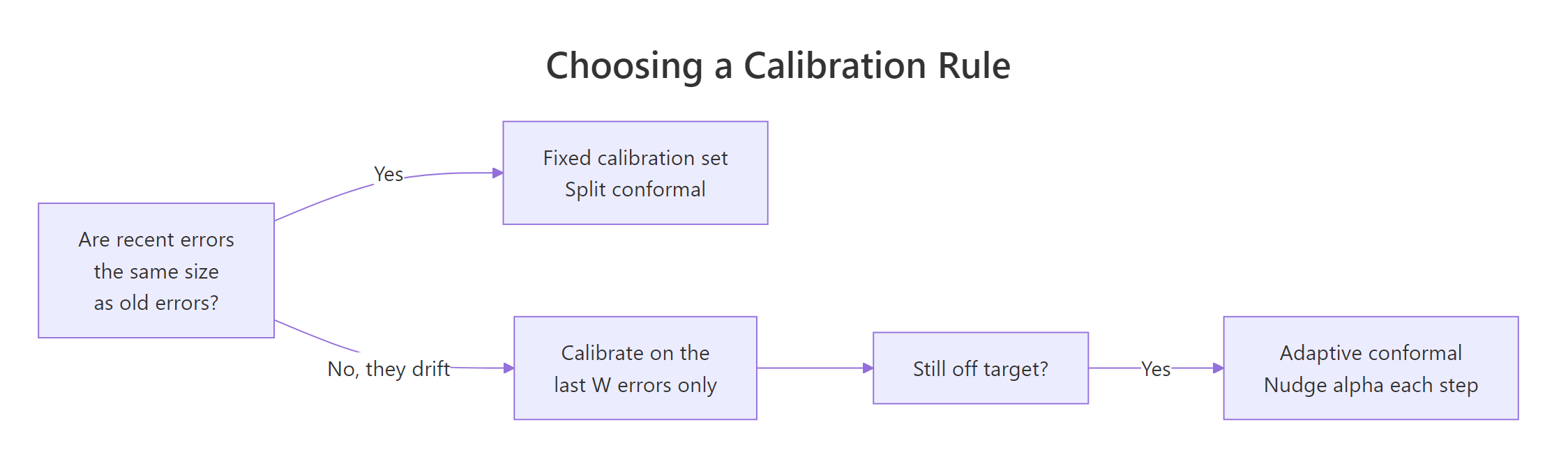
Figure 2: Which calibration rule to use once the errors start drifting.
Fix one: a rolling calibration window
Instead of freezing the calibration set at the first 60 forecasts, recompute the quantile at every step from only the most recent W errors. The window slides forward with you, so when the model gets worse the interval widens automatically, and when it gets better the interval tightens.
The only change inside the loop is which errors feed the quantile: audit$err[(k - W):(k - 1)] is always the 40 most recent misses as of the moment you forecast, and the slice stops one step short of audit$err[k], the error you are trying to cover.
The interpretation is that coverage went from 85.3% to 97.1%, comfortably past the 95% target, and the price was width: 16,598 bottles against 10,342. That is uncomfortable, and it is also the truth. The static interval was not better, it was wrong. Once you insist on genuinely covering 95% of months on the later, harder part of this series, this is what it costs.
Notice the rolling version slightly overshoots. Forty recent errors is a small sample, so the quantile is jumpy and tends to land high. That is the second fix's job.
Fix two: adaptive conformal inference
A rolling window reacts to changes in error size, but it never checks whether it is actually hitting the target. Adaptive conformal inference, introduced by Gibbs and Candes, adds that feedback loop. It keeps a working error rate $\alpha_t$ that moves after every observation:
$$\alpha_{t+1} = \alpha_t + \gamma \left( \alpha - \mathbb{1}\{ y_t \notin C_t \} \right)$$
Where:
- $\alpha_t$ = the error rate the algorithm is currently using to pick the quantile
- $\alpha$ = the error rate you actually want, 0.05 here
- $\gamma$ = the step size, controlling how sharply it reacts
- $\mathbb{1}\{ y_t \notin C_t \}$ = 1 if the last interval missed, 0 if it covered
Read it as a thermostat. After a miss the bracket becomes $\alpha - 1$, a large negative number, so $\alpha_t$ drops and the next interval widens. After a hit the bracket is $\alpha$, a small positive number, so $\alpha_t$ creeps up and the interval tightens. Over time the two forces balance at the target rate.
The walk-through: a_use clamps the working rate into a legal range so a long run of hits cannot push it past 1. Everything else is the rolling window from before, except that the alpha fed to conf_q now changes every step, and the final line applies the thermostat.
The interpretation is that adaptive conformal delivered 95.6% coverage, closer to the 95% target than the rolling window's 97.1%, and it did so with a narrower average interval: 15,391 against 16,598. Better coverage and less width at the same time, because every stretch of covered months raised the working alpha, which narrowed the next interval instead of leaving it too wide.
The working rate ranged from 0.040 up to 0.1175. Each covered month adds gamma * alpha, which is 0.0025, so a run of hits walks the rate up toward 0.12 and narrows the interval; each miss subtracts gamma * (1 - alpha), which is 0.0475, nineteen times larger, so one miss undoes nineteen hits. You asked for 5% and internally the algorithm spent most of its time asking for something else, which is how it delivered 5% on the outside.
Try it: The window length is a real tuning knob. Try W = 20 instead of 40 and see what a shorter memory does to coverage.
Click to reveal solution
Explanation: A 20-error window covers 98.5%, even further above target than the 40-error window. With only 20 scores the 95% conformal rank is the largest one, so the interval is set by the single worst recent miss. Short windows adapt faster but get noisier, which is exactly the pressure adaptive conformal relieves.
How do you put an interval on a model that has no interval formula?
Everything so far has been an improvement on an interval that already existed. Now the case where conformal prediction is not an improvement but the only option available.
A random forest forecaster returns a number. That is all. There is no error term to be normal, no likelihood, no closed-form variance of the prediction. The same is true of gradient boosted trees, of nearest-neighbour forecasters, and of most machine learning methods people now point at time series. Conformal prediction never looks inside the model, only at the errors it made, so a missing variance formula costs it nothing.
To use a forest we first have to reshape the series into a table, since trees work on rows of features rather than on ordered observations. Each row gets the value we want to predict plus a few of its own past values as columns.
Each row now says: here is a month's sales, here is last month, here is the same month a year ago, and here is the month before that a year ago. complete.cases() drops the first 13 rows where those lags do not exist yet, leaving 163 usable rows.
Now train the forest on the first 48 rows and let it predict everything after.
predict(rf, rf_live) gives one number per month and nothing else. There is no $lower or $upper to ask for, because the forest has no theory of its own uncertainty. Everything we need is in the err column.
The conformal step is now literally identical to the one we ran on ETS. That is the point.
The interpretation: a model that offered no interval at all now has one covering 96.0% of months, from twelve lines of code that never once referenced how the forest works. Swap randomForest for any other point forecaster and not a single line of the conformal step changes.
Look at the width, though: 21,528 bottles against ETS's 16,598 under the identical procedure. The forest's average miss is 2,647 bottles while ETS's is 2,498 across its full audit, so the forest is genuinely the weaker model here, and the wider interval is a direct reading of that.
Try it: Confirm the comparison for yourself. Compute the ETS model's mean absolute error across its full audit and check it against the forest's 2,647.
Click to reveal solution
Explanation: ETS is about 6% more accurate on average, and its conformal interval is about 23% narrower. The gap in interval width is larger than the gap in average error because the conformal quantile responds to the worst recent misses, not to the average, and the forest's bad months are worse.
How do you run conformal prediction with the conformalForecast package?
Building it by hand was the point of this page, because you now know exactly what every number means and where it can fail. For production work there is a package: conformalForecast by Xiaoqian Wang and Rob Hyndman, which implements classical conformal prediction, adaptive conformal prediction, conformal PID control, and the autocorrelated multistep method from their 2024 paper.
It is not available in this page's in-browser R, so run the block below in your own R session after install.packages("conformalForecast"). The output shown is real, captured from a local run against the same wine series.
library(conformalForecast)
library(forecast)

sales <- wineind
etsfun <- function(x, h, level) forecast(ets(x), h = h, level = level)

fc <- cvforecast(sales, forecastfun = etsfun, h = 6, level = 95,
                 forward = TRUE, initial = 48, window = NULL)

scpfc <- scp(fc, symmetric = TRUE, ncal = 60, rolling = TRUE)
coverage(scpfc, level = 95)
#>       h=1       h=2       h=3       h=4       h=5       h=6
#> 0.9411765 0.9393939 0.9218750 0.9516129 0.9333333 0.9482759

width(scpfc, level = 95)
#> Mean width:
#>      h=1      h=2      h=3      h=4      h=5      h=6
#> 13793.47 13863.18 14139.54 14735.21 14291.46 14539.26
Three functions do the work. cvforecast() runs the rolling-origin loop we wrote by hand, calling your forecasting function at every origin. scp() performs split conformal prediction, where ncal = 60 sets the calibration size and rolling = TRUE switches on the sliding window we built in the previous section. coverage() and width() then score the result.
The interpretation matters as a cross-check: the package reports 92% to 95% coverage at widths near 14,000, and our hand-rolled rolling window reported 97.1% at 16,598. Same ballpark, and the differences are explained by details we now understand, mainly that scp() recalibrates on a rolling basis from the first available origin rather than from a fixed cutoff. Because you built the method yourself, a discrepancy like that is a question you can answer instead of a black box you have to trust.
scp(), it offers acp() for adaptive conformal prediction, pid() for conformal PID control, and the autocorrelated multistep method that exploits a specific fact about forecast errors: optimal h-step errors are serially correlated up to lag h-1, so multistep intervals can be sharpened by modelling that correlation instead of ignoring it.Try it: The package asks you to choose ncal. Use the rank rule to find the smallest calibration window that can produce a finite 95% interval from real error data, so you know the floor before you tune.
Click to reveal solution
Explanation: 19, matching the algebra from the earlier section. Anything smaller and conf_q() returns Inf, which is the honest answer: with fewer than 19 held-out errors there is no finite 95% interval that the rank rule will vouch for. Set ncal well above the floor so the quantile is not pinned to your single worst observation.
Complete Example: a reusable conformal_forecast() function
Here is everything on this page collapsed into one function you can point at any series and any point forecaster. It runs the rolling-origin audit, calibrates on the most recent errors at every horizon, and returns a forecast table with honest bounds.
The model_fun argument is the whole design. It takes a series and a horizon and returns point forecasts, which means the forest from two sections ago, an ARIMA, a seasonal naive benchmark, or your own function all drop in without touching the conformal machinery. tail(errs, window) keeps only the most recent errors so the calibration stays current, and apply(..., 2, conf_q) calibrates each horizon on its own column.
auto.arima, to snaive, or to the random forest is a change to ets_frozen alone. Keeping that boundary clean is what lets you swap models without ever revalidating the interval code.Compare these bounds to the ETS output we started with. Back then the model claimed September 1994 would land between 20,464 and 29,013, a span of 8,549 bottles. The conformal version says between 17,711 and 32,370, a span of 14,660. That is the same forecast with the uncertainty told straight.
Practice Exercises
Exercise 1: Build a rolling 80% conformal interval end to end
Earlier the static 80% conformal interval covered only 44.1%. Rebuild it with a rolling 40-error window over the same test period (rows 61 onward of audit) and report the coverage and mean width. Use my_ prefixed variables so you do not overwrite anything above.
Click to reveal solution
Explanation: The rolling window lifts coverage from 44.1% to 73.5%, a huge repair, but it still falls short of 80%. Lower confidence levels are harder to hit with a sliding window because they depend on the middle of the error distribution, which moves around more than the tail does. This is a case for adaptive conformal inference rather than a longer window.
Exercise 2: Diagnose a rolling window that under-covers
Apply per-horizon rolling conformal prediction to AirPassengers for horizons 1 to 3 at 95%, using the err_a matrix already in memory. Measure coverage with W = 40, then again with W = 20, and explain which wins and why.
Click to reveal solution
Explanation: The shorter window wins clearly, about 91% against 78% to 86%. Airline passenger volumes roughly tripled over the sample, so the model's errors grow fast, and a 40-month memory is still full of errors from a much smaller airline industry. On a rapidly drifting series a short window is not noisier in any way that matters, it is simply more current. Neither window reaches 95%, which tells you the frozen model itself needs refitting.
Exercise 3: Give the interval two different sides
Every interval so far has been symmetric, using a single quantile of absolute errors. That is wasteful when a model misses harder in one direction than the other. Build an asymmetric 90% interval that calibrates the upper and lower offsets separately from the signed errors, using a rolling 40-error window, and compare its coverage and width to the symmetric version.
Click to reveal solution
Explanation: The asymmetric interval hits 89.8% against a 90% target while the symmetric one manages 86.4%, and it costs only 5% extra width. Splitting the budget lets each side find its own quantile, so a model that overshoots and undershoots by different amounts gets bounds that reflect that. The cost is that each side now calibrates on half the error budget, so you need a larger window before the tails are estimated reliably.
Frequently Asked Questions
Does conformal prediction work with ARIMA, Prophet, or a neural network?
Yes, and nothing in the recipe changes. The method needs a column of held-out errors and nothing else, so any function that takes a series and a horizon and returns numbers drops into the model_fun slot of conformal_forecast(). The random forest section is the proof: the same dozen lines wrapped an interval around a model that has no interval theory of its own.
How many calibration errors do I actually need?
For a 95% interval the hard floor is 19, because the rank rule asks for a sorted position that has to exist: with 19 scores it asks for the 19th, and with 18 it asks for a 19th that is not there. Sitting at the floor is a bad idea anyway, because the interval is then set by your single largest calibration error and jumps around whenever that error changes. Aim for several times the floor, and on a drifting series prefer a rolling window of roughly 40 recent errors to a long fixed one.
Is this the same as a bootstrap prediction interval?
No. A bootstrap interval resamples past residuals and simulates many possible futures through the model, so it still relies on the model being right about how errors propagate forward. Conformal prediction skips the simulation and reads a quantile straight off the errors the model actually made. Both deserve the rolling-origin audit from the first section, because only the audit tells you which one covers on your series.
Does conformal prediction make my forecast more accurate?
No. The point forecast is untouched, and only the interval around it changes. If the interval comes out wider than you expected, that is a measurement of the model you already had rather than a penalty the method imposes, and the only way to narrow it honestly is a better point forecast.
Why is my conformal interval the same width for every future month?
Because the absolute error score gives every future point the same treatment: one quantile, one half-width. That is reasonable when the model is equally accurate everywhere in the series, and wrong when it is not, for example if December is always harder to forecast than July. The two standard repairs are to divide each error by a predicted scale before taking the quantile, or to calibrate around a quantile regression instead, which is the conformalized quantile regression of Romano and colleagues listed in the references.
My coverage is still below target. What should I check first?
Drift, because it is the usual cause. Split the errors into consecutive blocks and compare their averages, exactly as the exchangeability section does; if the later blocks are larger, a fixed calibration set is describing an accuracy the model no longer has, and a rolling window plus the adaptive alpha update recovers most of the gap. If the blocks look similar, check that your calibration set is comfortably above the floor and that you used the rank rule rather than quantile().
Summary
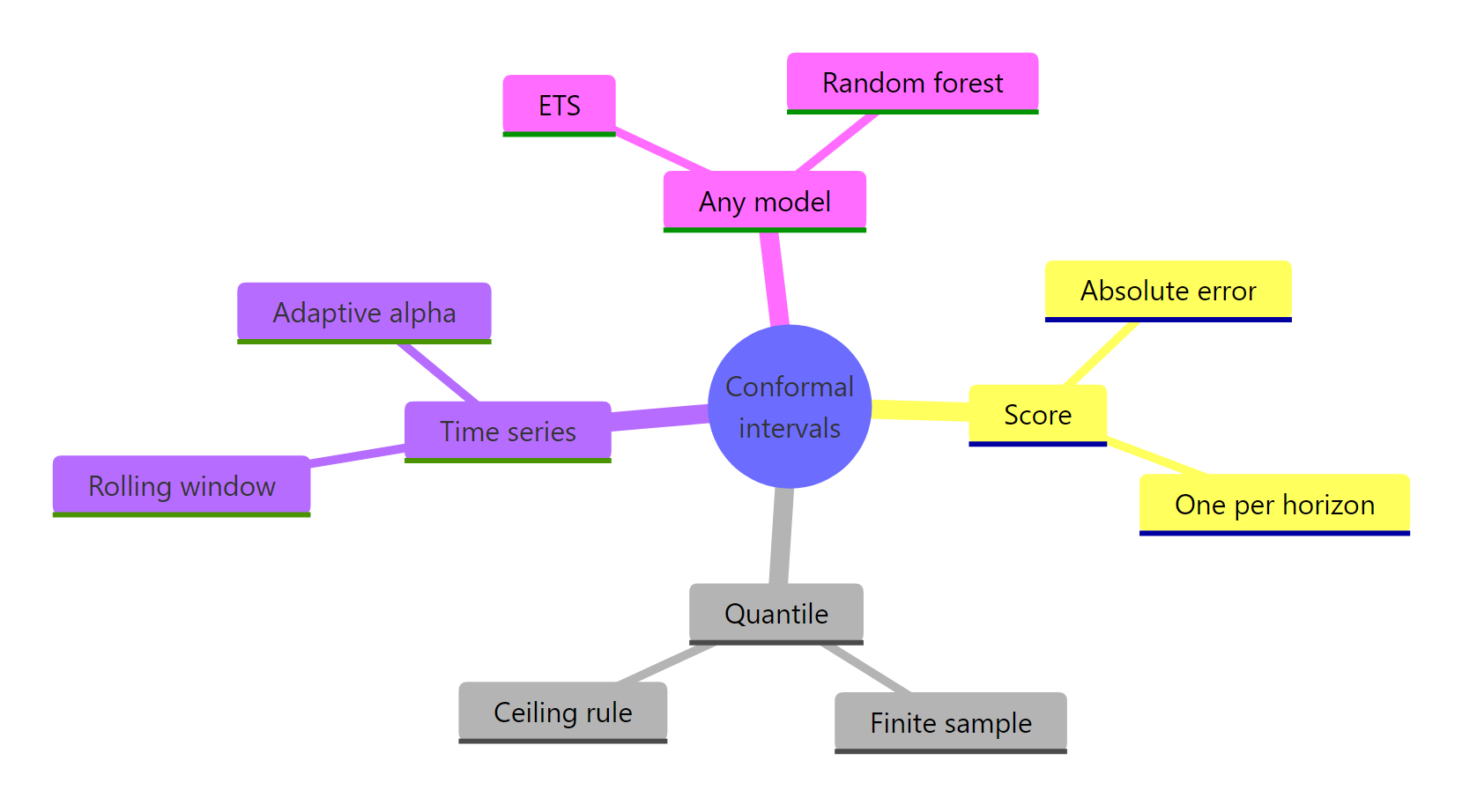
Figure 3: The four decisions behind every conformal forecast interval.
Every number below was measured on the wine sales series. The first four rows share the same ETS model and the same 68 held-out months, so they compare directly. The forest row uses a different model over a slightly longer span of months, so read it as a demonstration that the method attaches to anything, not as a like-for-like contest.
| Method | What it fixes | Measured coverage | Mean width |
|---|---|---|---|
| ETS parametric interval | Nothing, it is the baseline | 0.779 | 9,120 |
| Split conformal, fixed calibration | Drops the normality assumption | 0.853 | 10,342 |
| Rolling calibration window | Drops the stale-calibration problem | 0.971 | 16,598 |
| Adaptive conformal inference | Steers coverage back to target | 0.956 | 15,391 |
| Conformal around a random forest | Gives an interval to a model that had none | 0.960 | 21,528 |
The takeaways worth keeping:
- Audit before you trust. A nominal 95% interval covered 84% of months on an ordinary commercial series with a sensible model. One rolling-origin loop tells you where you stand.
- The recipe is four lines. Held-out absolute errors, sort, take rank $\lceil (n+1)(1-\alpha) \rceil$, add and subtract. There is nothing else to it.
- Use the rank, never
quantile(). The interpolating version under-covered by nearly four points in a controlled simulation, and the gap is worst exactly when calibration sets are small. - Measure whether your errors grow with the horizon. From one month ahead to six, they grew 78% on airline passengers and stayed flat on wine sales. Calibrating per horizon is right either way.
- Exchangeability is what breaks on time series. Errors on this series grew 2.4 times from the first quarter of the sample to the last, which is why fixed-calibration conformal reached only 85%.
- A rolling window plus adaptive alpha is the working recipe. Together they delivered 95.6% coverage at a narrower width than the rolling window alone.
- Conformal is the only interval available for most machine learning forecasters. It attaches to any point forecast, and when the model is weak it tells you so with a wider interval rather than hiding it.
References
- Vovk, V., Gammerman, A., & Shafer, G. Algorithmic Learning in a Random World, 2nd Edition. Springer (2022). The foundational text on conformal prediction. Link
- Shafer, G., & Vovk, V. A Tutorial on Conformal Prediction. Journal of Machine Learning Research, 9, 371-421 (2008). Link
- Lei, J., G'Sell, M., Rinaldo, A., Tibshirani, R. J., & Wasserman, L. Distribution-Free Predictive Inference for Regression. Journal of the American Statistical Association, 113(523), 1094-1111 (2018). The split conformal method used throughout this page. Link
- Gibbs, I., & Candes, E. Adaptive Conformal Inference Under Distribution Shift. NeurIPS (2021). The source of the alpha update rule in the adaptive section. Link
- Wang, X., & Hyndman, R. J. Online conformal inference for multi-step time series forecasting. arXiv:2410.13115 (2024). Establishes that optimal h-step errors are serially correlated up to lag h-1, and introduces the AcMCP method. Link
- conformalForecast: Conformal Prediction Methods for Multistep-Ahead Time Series Forecasting. CRAN package documentation. Link
- Romano, Y., Patterson, E., & Candes, E. Conformalized Quantile Regression. NeurIPS (2019). How to make conformal interval widths vary with the input rather than staying constant. Link
- Hyndman, R. J., & Athanasopoulos, G. Forecasting: Principles and Practice, 3rd Edition. OTexts (2021). Chapter 5.5 covers parametric prediction intervals and the assumptions this page tests. Link
Continue Learning
- Gradient Boosting for Time Series in R builds the boosted-tree forecaster that most needs a conformal interval, since it returns a point forecast and nothing else.
- Global Forecasting Models in R trains one model across many series at once, which gives you a much larger pool of calibration errors to conformalize with.
- Feature Engineering for Forecasting in R goes deeper on the lag table we built for the random forest, including rolling statistics and calendar features.