TBATS in R: Forecast Multiple Seasonalities
TBATS is a forecasting model in R's forecast package built for series that repeat on more than one clock at once, like hourly data that cycles every day and every week. It swaps the usual seasonal indices for trigonometric waves, and that one substitution is what lets it handle the long, multiple, and fractional seasonal periods that ets() and auto.arima() simply refuse.
Everything below uses only the forecast package and datasets that ship with it, so you can run every block right here in the page without installing or downloading anything.
What makes seasonality "complex", and why does ets() refuse to model it?
Most forecasting tutorials assume your data repeats on exactly one schedule: monthly sales that cycle every 12 months, quarterly revenue that cycles every 4 quarters. Real high-frequency data is rarely that tidy. Electricity demand rises and falls across the day, and it also follows a completely separate weekday-versus-weekend rhythm. Watch what R's standard seasonal model does when you hand it a series like that.
Three things happened there. length() tells us there are 4032 observations. The msts attribute reports that this series carries two seasonal periods, 48 and 336. And ets() returned a model whose third letter is N.
That N is the whole problem. In R's ETS notation the three letters describe the error, trend, and seasonal components, so ETS(A,Ad,N) means additive error, additive damped trend, and no seasonal component at all. Run that block and you will also see R print a warning: it cannot handle data with frequency greater than 24, so it ignored the seasonality and fitted a non-seasonal model instead. It did not stop with an error. It handed back a perfectly usable model that has no seasonal component in it, which means it dropped the strongest signal in the data.
The 48 and 336 are not arbitrary. The series is recorded every half hour, so 48 half-hours make one day and 336 make one week. Both cycles are genuinely present, and we can pull them apart to prove it.
mstl() is a multi-seasonal decomposition: it peels the series into a trend plus one column per seasonal period, leaving the unexplained part as a remainder. It found both cycles and named them after their periods. The averages say the daily swing moves demand by about 4,206 MW on average while the weekly swing moves it by about 2,379 MW. The daily cycle is bigger, but the weekly one is far too large to discard, which is exactly what ets() just did.
This is what forecasters mean by complex seasonality, and it shows up in three flavours:
- Multiple seasonal periods. Hourly data repeats every 24 hours and every 168 hours. Daily retail data repeats weekly and annually.
- Long seasonal periods. Rob Hyndman notes that
ets()caps out at a period of 24, andArima()will usually run out of memory once the seasonal period goes past about 200. A yearly cycle in daily data has a period of 365. - Non-integer seasonal periods. A year is not 52 weeks, it is 52.18 weeks. It is not 365 days either, it is 365.25. Classical seasonal models need a whole number.
TBATS exists to solve exactly these three problems, and the rest of this tutorial builds it up from that starting point.
Try it: The taylor series is recorded every half hour. Work out how many whole days of data it covers, and store the answer in ex_days.
Click to reveal solution
Explanation: length(taylor) gives 4032 observations, and dividing by the 48 half-hours in a day gives 84 days, which is 12 complete weeks. That is why the 336-period weekly cycle is estimable here: the data contains 12 full repetitions of it.
What does TBATS stand for, and what does the "T" actually do?
TBATS is an acronym, and each letter names a component the model bolts on. Reading them in order tells you exactly what the model does to your data.

Figure 1: Each letter of TBATS adds one stage to the model, applied in this order.
| Letter | Stands for | What it does |
|---|---|---|
| T | Trigonometric | Represents each seasonal cycle as a sum of sine and cosine waves instead of one value per slot |
| B | Box-Cox | Optionally transforms the data to stabilise variance that grows with the level |
| A | ARMA | Models any pattern still left in the residuals with an ARMA process |
| T | Trend | A local level plus an optional slope, which can be damped |
| S | Seasonal | The seasonal components themselves, one per period |
Two words in that table will keep coming back, so pin them down now. The residuals are what is left of your data once the model's own fitted values are subtracted, one leftover number per time point. Autocorrelation means those leftovers are still predictable from each other: if a high leftover tends to be followed by another high one, there is structure the model has not accounted for. The A in TBATS exists to model whatever autocorrelation the other components leave behind.
The history explains the odd letter ordering. De Livera, Hyndman and Snyder first defined a model called BATS, which stands for Box-Cox transform, ARMA errors, Trend and Seasonal components. BATS still used the classical one-value-per-slot seasonality. They then swapped that seasonality for a trigonometric version and stuck a T on the front. TBATS is literally BATS with trigonometric seasonality.
So the interesting letter is the leading T. Here is what "trigonometric" means in practice. Any repeating shape, however lumpy, can be rebuilt by adding together sine and cosine waves of different speeds. The slowest wave completes one cycle per period. Each faster wave completes one more cycle than the one before it. Each of these waves is called a harmonic.
The 2 * pi * j / m term walks once around a full circle as j runs from 1 to m. Multiplying by 1 gives a wave that peaks once per day. Multiplying by 2 makes it go round twice as fast, so it peaks twice per day. You can see it in the numbers: wave1 is still climbing at position 6, while wave2 has already peaked at position 3 and come back to zero at position 6.
Add a handful of these waves together with the right weights and you can approximate any daily pattern you like. That is the trick. Instead of storing 24 separate values, TBATS stores a weight for each harmonic. Instead of 336 values for a weekly cycle, it might store weights for just 6 harmonics.
The seasonal equations (skip this if you only want the code)
If you are not interested in the math, jump to the next section. The code above is all you need to use the model.
Each seasonal component is the sum of its harmonics, where $k_i$ is the number of harmonics kept for period $i$:
$$s_t^{(i)} = \sum_{j=1}^{k_i} s_{j,t}^{(i)}$$
Each harmonic is a point rotating around a circle. Two equations move it one step per time period, and both get nudged by the current error so the seasonal shape can drift:
$$s_{j,t}^{(i)} = s_{j,t-1}^{(i)}\cos \lambda_j^{(i)} + s_{j,t-1}^{*(i)}\sin \lambda_j^{(i)} + \gamma_1^{(i)} d_t$$
$$s_{j,t}^{(i)} = -s_{j,t-1}^{(i)}\sin \lambda_j^{(i)} + s_{j,t-1}^{(i)}\cos \lambda_j^{(i)} + \gamma_2^{(i)} d_t$$
Where:
- $s_{j,t}^{(i)}$ is the level of harmonic $j$ of seasonal period $i$ at time $t$
- $s_{j,t}^{*(i)}$ is its companion, the growth in that level, needed to let the shape change over time
- $\lambda_j^{(i)} = 2\pi j / m_i$ is the angle the harmonic advances each step, with $m_i$ the seasonal period
- $\gamma_1^{(i)}$ and $\gamma_2^{(i)}$ are smoothing parameters that control how fast the season is allowed to drift
- $d_t$ is the ARMA error process, the
Ain TBATS
Two consequences fall straight out of these equations. First, $m_i$ appears only inside $\lambda_j^{(i)} = 2\pi j / m_i$, as a plain division. Nothing requires it to be a whole number, which is how TBATS handles a period of 52.18. Second, if you set both smoothing parameters to zero the seasonal shape freezes and never changes, which reduces TBATS to ordinary harmonic regression. The $\gamma$ terms are precisely what makes TBATS seasonality dynamic.
The B for Box-Cox is a variance-stabilising transform applied before any of this, controlled by a parameter $\omega$ that R calls lambda:
$$y_t^{(\omega)} = \begin{cases} (y_t^{\omega}-1)/\omega & \omega \neq 0 \\ \log y_t & \omega = 0 \end{cases}$$
Try it: Build the third harmonic of the daily cycle, the wave that completes three full cycles per day, and store it in ex_wave3.
Click to reveal solution
Explanation: Changing the multiplier from 2 to 3 makes the wave complete three cycles per period, so it reaches its peak of 1.000 at position 2 and is already back to zero at position 4. Higher harmonics capture finer, faster wiggles in the seasonal shape.
How do you fit your first TBATS model in R?
Before tackling two seasonal cycles, fit TBATS to a plain single-season series so you can see the machinery clearly. USAccDeaths is monthly accidental deaths in the US, which ships with base R and has an obvious 12-month cycle.
You gave tbats() one argument plus a speed flag and it searched for you. It tried the model with and without a Box-Cox transform, with and without a trend, with and without damping, and with different numbers of harmonics, then kept whichever combination scored the lowest AIC. AIC is a single number that rewards fitting the data closely and charges a penalty for every parameter used to do it, so lower is better, and a model only earns an extra parameter if that parameter buys more fit than it costs.
The seed states are the starting values the model needs for every component it tracks, printed here as one column. Count them: there are exactly 11, and that is not a coincidence. One is for the level, the model's running estimate of where the series sits once season and noise are set aside, and the other 10 are 2 apiece for the 5 harmonics it chose. This is the parsimony argument from the last section, made concrete. A classical seasonal model would have needed 12 seasonal values here, and 12 is small. The gap becomes enormous when the period is 336.
Alpha is the smoothing parameter for the level, and the two Gamma values control how fast the seasonal shape is allowed to drift. Both gammas are tiny, around 0.01, which tells you the seasonal pattern in this series is almost fixed from year to year.
tbats() spins up parallel workers whenever the series is longer than 1000 points. The setup overhead often costs more than it saves, and the parallel path is known to hang in some environments. Turn it on deliberately, not by accident.Now the obvious question: is the trigonometric version actually better than the classical one? bats() takes exactly the same arguments and fits the classical-seasonality version, so you can compare directly.
Lower AIC is better, so TBATS wins by about 6 points on this series. It described the same seasonal pattern using 5 harmonics where BATS spent 12 seasonal values, and the penalty for those extra parameters is what pushed BATS behind.
Try it: The automatic search decided not to apply a Box-Cox transform here. Force it on with use.box.cox = TRUE, then check the AIC to see whether the search was right.
Click to reveal solution
Explanation: The chosen lambda is 0.0004, which is effectively zero and therefore effectively a log transform. The AIC rose from 1132.92 to 1135.44, so the transform cost a parameter without buying any fit. The automatic search was right to leave it off.
How do you read a TBATS model string?
The first line of that output, TBATS(1, {0,0}, -, {<12,5>}), is the model's entire specification compressed into one line. Learning to read it is the fastest way to understand what R chose for you.
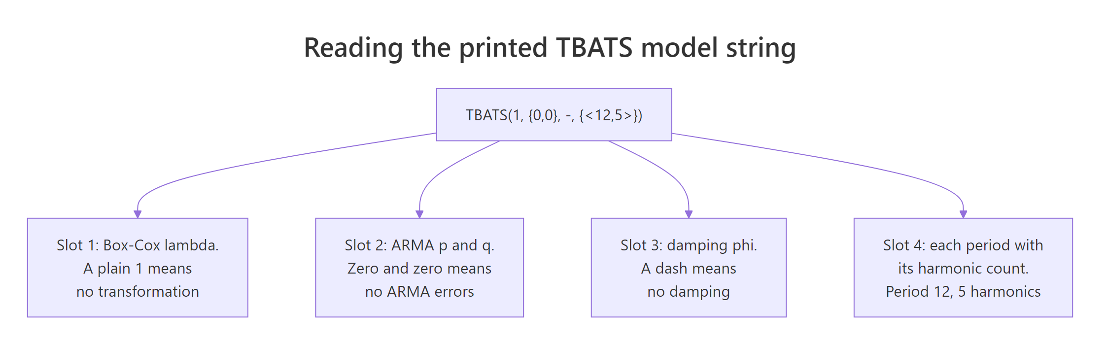
Figure 2: The four slots R prints in a TBATS model string.
| Slot | Example value | Meaning |
|---|---|---|
| 1 | 1 |
The Box-Cox lambda. A bare 1 means no transformation was applied |
| 2 | {0,0} |
The ARMA orders {p,q} on the errors. {0,0} means no ARMA errors |
| 3 | - |
The damping parameter phi. A dash means damping was not used |
| 4 | {<12,5>} |
One <period, harmonics> pair per seasonal cycle. Here: period 12, 5 harmonics |
Do not take my word for it. Every slot corresponds to a field on the fitted object, so you can read them off directly.
Both lambda and damping.parameter are NULL, which is why slots 1 and 3 printed the placeholder 1 and -. The period and harmonic count are stored separately as seasonal.periods and k.vector, then printed together as <12,5>. And with zero AR coefficients stored, slot 2 shows {0,0}.
That third slot causes more confusion than the rest combined.
use.trend and the presence of a Beta parameter to find out about the trend.Proving it takes one line. Force damping on and watch the dash turn into a number.
A phi of 0.929 means each step of the trend is multiplied by 0.929 as you forecast further out, so the slope flattens toward zero instead of running away. Values close to 1 damp slowly, values near 0 damp aggressively.
Try it: Fit that damped model again, keep it in ex_damped, and print its model string with as.character(). Predict what will be in slot 3 before you run it.
Click to reveal solution
Explanation: Slot 3 changed from - to 0.929, the rounded damping parameter. Everything else stayed the same: no Box-Cox, no ARMA errors, still 5 harmonics on a period of 12.
How do you model two seasonal cycles at once?
Now for the case TBATS was actually invented for. We will simulate five weeks of hourly page views for a website, with a daily rhythm that slowly grows stronger and a weekend lift on top of it. Simulating means we know the right answer, which makes it easy to judge whether the model found it.
The %% operator gives the remainder and %/% gives the integer quotient, so together they convert a running hour counter into "hour of day" and "day of week". %in% returns TRUE wherever a value is one of the ones listed, so day_of_week %in% c(5, 6) is TRUE on the two weekend days, and multiplying that by 60 turns it into a flat 60-view lift on those days only. The daily amplitude starts at 80 and grows by 6 each week, so by week five the daily swing is 30 percent larger than it was in week one. That growing amplitude is a drifting season, which is precisely the situation TBATS is designed for.
Next we tell R about both cycles. A regular ts object holds only one frequency, so the forecast package supplies msts() for multi-seasonal series.
We held out the final week so there is honest data to score against later. The object is now class msts, and it carries both periods: 24 for the daily cycle and 168 for the weekly one.
Before we fit anything, one detail about msts() is worth seeing, because it goes wrong silently and the help page does not flag it.
Look carefully. We asked for a period of 52.18, and we got back an object of class ts, not msts, with a frequency of 52. The fractional part was silently discarded. msts() only creates a genuine multi-seasonal object when you give it more than one period; with a single period it falls back to a plain ts, and a plain ts frequency must be a whole number.
tbats(ts(x), seasonal.periods = 52.1786). Routed through msts() the same cycle silently becomes 52, and an error of 0.18 per year accumulates to nearly a full week of drift per decade. msts() earns its place only when you have two or more periods.With the data correctly declared, the fit itself is one call.
Slot 4 now holds two pairs instead of one: <24,7> and <168,6>. The model kept 7 harmonics to describe the daily cycle and 6 for the weekly one. There are also two Gamma-1 values and two Gamma-2 values, one pair per seasonal component, because each cycle drifts at its own rate.
I switched off Box-Cox and ARMA errors here purely for speed, and we will switch ARMA back on in the next section once you have seen why it matters.
use.box.cox = FALSE and use.arma.errors = FALSE are the two biggest speed levers, and use.arma.errors = FALSE alone roughly halves the work.Try it: The model reports its seed states. Count them with nrow(fit_views$seed.states) and check the count against the formula 1 + 2 * sum(k), where k is the harmonic counts in fit_views$k.vector.
Click to reveal solution
Explanation: 27 states break down as 1 for the level plus 2 for each of the 13 harmonics, since 7 plus 6 is 13. Compare that with a classical seasonal model, which would need 24 values for the daily cycle and 168 for the weekly one, so 192 in total. TBATS described the same structure with 27.
How do you check whether a TBATS model is any good?
A model that fits is not the same as a model that forecasts. Start by predicting the week we held out and scoring the result.
accuracy() scores the fitted values against the training data on the first row and the forecasts against the held-out week on the second. The test MAPE of 3.29 percent means the forecasts were typically about 3.3 percent away from the truth. RMSE is the same idea in the original units rather than percentages, so the test RMSE of 16.99 says the typical miss was about 17 page views, only slightly worse than the 14.78 the model managed on the data it trained on. A small gap like that says the model generalised rather than memorised.
One number on that first row is a warning sign though. ACF1 is the autocorrelation of the residuals at lag 1, and 0.23 is high. If the model had extracted all the structure, the leftovers would look like random noise with no autocorrelation. Let us test that properly.
The Ljung-Box test asks a single question: are these residuals indistinguishable from random noise? A small p-value says no. Here the p-value is below 2.2e-16, so the residuals still contain plenty of structure the model has not captured.
That is a real failure, not a mistake in the code, and it has an obvious cause: we turned off ARMA errors to make the fit faster. Modelling exactly this kind of leftover autocorrelation is the entire job of the A in TBATS. Switch it back on.
Slot 2 changed from {0,0} to {2,0}, meaning R added an AR(2) process to the errors: each error is now predicted from the two errors immediately before it, weighted by the coefficients 0.209 and 0.136. The AIC improved from 8059.1 to 8031.3. Now re-run the residual test on the new model.
The test statistic fell from 478.26 to 225.19, so the ARMA component absorbed more than half the leftover autocorrelation. The p-value is still small, meaning some structure remains, which is common with 672 observations because the test gets very sensitive at that sample size.
So the AIC improved and the residuals improved. Both of those were measured on the training data, though. Score the two models on the week we held out instead.
The verdict flips. The model that scored better on AIC forecast slightly worse on data it had never seen. AIC is computed entirely from the training data, so it can prefer a model that the future does not. When the two disagree, trust the holdout.
tbats() returns during its internal search, and that search never sees your test set. Always hold out a final stretch of data and score forecasts against it, exactly as we did with views_test.checkresiduals() reports "Model df: 0" for TBATS objects. It does not subtract the model's estimated parameters from the degrees of freedom the way it does for ARIMA fits, so the p-value is more likely to flag a problem than it should be. Read it as a directional signal rather than a formal test.You can also pull the fitted seasonal pieces apart to see what the model learned.
season1 is the 24-hour cycle and season2 is the 168-hour one, matching the order you passed to msts(). At the very first observation the level sits at 425.59, the daily cycle pulls it down by 58.17 because it is the middle of the night, and the weekly cycle nudges it up by 5.71.
use.box.cox = FALSE, so the scales happen to agree, but check fit$lambda before you trust the arithmetic.Try it: Work out how wide each seasonal component swings by taking the range of every column of tbats.components(fit_views). Which cycle dominates?
Click to reveal solution
Explanation: diff(range(z)) is the distance from a column's smallest value to its largest. The daily cycle swings across 193.2 page views while the weekly cycle covers only 75.8, so the daily rhythm dominates. The level barely moves at 20.0, which is right, since we simulated no real trend.
When should you not use TBATS?
TBATS has a reputation as the automatic answer for messy seasonal data. It is not, and knowing its limits will save you more time than knowing its options. Start with the limitation that bites hardest in practice.
We passed an external regressor and tbats() accepted it without complaint. The resulting model string is the same one we got without the regressor, and identical() confirms the two AIC values match to the last digit. Nothing about the fit changed, and nothing was printed to say the argument had been dropped.
auto.arima() with fourier() terms plus an xreg matrix instead, which handles multiple seasonality and covariates together.The second limitation is that TBATS frequently loses. Let us benchmark it honestly against three alternatives on the same held-out week. The third of them needs a word of introduction: fourier() builds exactly the sine and cosine harmonics we constructed by hand earlier, K of them for each seasonal period, and hands them to auto.arima() as ordinary regressor columns. That gives ARIMA multiple seasonality too, but with the harmonic weights held fixed rather than allowed to drift.
TBATS came third. stlf(), which runs a multi-seasonal STL decomposition and then applies ETS to what remains, beat it by 15 percent and finished in a fraction of the time. Even snaive(), which does nothing more sophisticated than repeating last week, edged it out.
This is not a fluke, and the reason is instructive. Our simulated weekly pattern is a fixed weekend lift that never changes shape, and both periods are exact whole numbers. Under those conditions the drifting seasonality TBATS pays parameters for buys nothing, while STL recovers the same fixed shape with a smoother that costs no model parameters at all.
So when does TBATS actually earn its keep? When the seasonal period is not a whole number. Here is weekly data whose true annual cycle is 365.25 / 7 = 52.1786 weeks, which no ts object can represent.
Note how the model was specified: a plain ts() for the data and the fractional period handed straight to tbats() via seasonal.periods, exactly as the earlier warning prescribed. Slot 4 confirms it worked, showing <52.18,3> rather than the <52,...> you would have got by routing through msts(). Three harmonics were enough to describe the annual shape.
The ranking flipped. TBATS now wins, and snaive() falls from second place to last, with more than twice the error of the winner. The reason is that every alternative had to round the period to 52, so their seasonal pattern slips by 0.18 weeks per year. Over the five-year training window that accumulates to almost a full week of drift, and their forecasts arrive out of phase. TBATS modelled 52.1786 directly and stayed aligned.
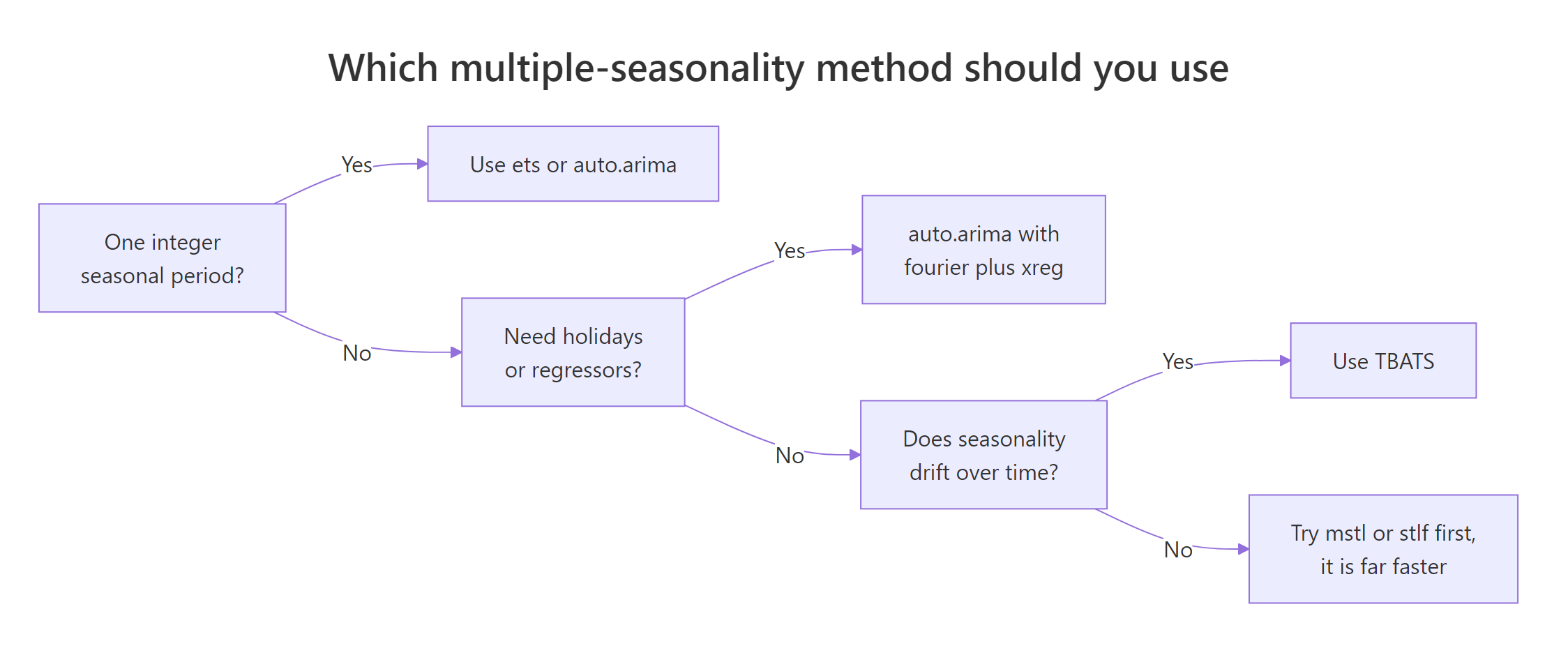
Figure 3: TBATS is one of four routes to a multiple-seasonality forecast.
Putting the limitations together:
- It is slow. Fitting involves a search over transforms, trend options and harmonic counts, each requiring a full optimisation. Expect seconds on small series and minutes on long ones.
- It ignores covariates. No holidays, no promotions, no weather, and no warning that they were dropped.
- It is univariate. One series at a time, with no cross-series information.
- It is hard to interpret. Harmonic weights do not map onto anything a stakeholder recognises, unlike a seasonal index that says "December is 40 percent above average".
- It is absent from fable. The modern tidyverts successor to
forecastdoes not implement TBATS, soforecast::tbats()remains the canonical route.
Try it: Add classical bats() to the weekly comparison. It cannot represent 52.18, so fit it on sales_52 and see how it scores.
Click to reveal solution
Explanation: BATS scored 19.71, worse than every method in the table. Its model string shows {52}, a bare integer period with no harmonic count, because classical seasonality stores one value per slot and slots must be whole numbers. It is stuck with the same rounding error as the others, without STL's flexible smoother to compensate.
Complete Example: an end-to-end weekly forecast
Here is the whole workflow in one place, on the fractional-period sales series where TBATS is the right tool. Split, fit, diagnose, forecast, then score.
This time we left use.arma.errors at its default of TRUE, and the search decided no ARMA component was worth keeping, so slot 2 stayed at {0,0}. The residual test now passes comfortably with a p-value of 0.497, meaning the leftovers are indistinguishable from noise. Compare that with the hourly model earlier, which failed the same test badly. This is what a well-specified TBATS model looks like.
A MAPE of 1.16 percent over a full year ahead is a strong result. The last line checks something the accuracy table never reports: how often the held-out values actually landed inside the stated 95 percent interval. We got 92.3 percent, a little below the promised 95, so the intervals are marginally too narrow here rather than too wide.
That is worth flagging because the standard advice, repeated from the FPP textbook, is that TBATS intervals tend to be far too wide. On this series they were slightly too narrow. Measure your own rather than assuming.
The dark band is the 80 percent interval and the lighter one the 95 percent interval. Both widen as the horizon grows, which is exactly what they should do: uncertainty compounds the further ahead you look.
Practice Exercises
These combine several ideas from the tutorial. Use the variable names given so nothing you write overwrites the objects above.
Exercise 1: Fit and decode a model on real wine data
wineind ships with the forecast package and holds monthly Australian wine sales. Fit both TBATS and BATS to it, compare their AIC values, then decode the TBATS model string slot by slot. This model uses more slots than any example above, so read it carefully.
Click to reveal solution
Explanation: TBATS wins on AIC, 3649.5 against 3670.5. Its model string uses every slot: a lambda of 0 means a log transform was applied, {1,0} means AR(1) errors with no MA part, 0.953 is a damping parameter, and <12,5> is the 12-month cycle described by 5 harmonics. Contrast that with the BATS string, where {12} is a bare period with no harmonic count, because classical seasonality has no harmonics to report.
Exercise 2: Measure the cost of the msts trap
Earlier you saw that msts(x, seasonal.periods = 52.18) silently rounds down to 52. Now put a number on the damage. Fit the sales series both ways, show that the model strings differ, and compare their held-out RMSE.
Click to reveal solution
Explanation: The model strings tell the story before the RMSE does. The msts() route produced <52,7>, a whole-number period needing 7 harmonics to chase a shape that keeps sliding out of phase. The direct route produced <52.18,3> and described the same cycle with 3. The RMSE cost is modest here at 8.54 against 8.29, roughly 3 percent, because five years is a short training window. Extend the series and the phase error accumulates, widening the gap.
Exercise 3: Write a function that picks the better model
The benchmarks showed that TBATS wins on one series and loses on another, so the honest workflow is to test rather than assume. Write pick_model(train, test, h) that fits both TBATS and stlf() to train, scores both against test, and returns the two RMSE values. Then run it on both series from this tutorial.
Click to reveal solution
Explanation: The function reproduces both verdicts from the benchmarks above, and the weekly one adds something new. TBATS wins there at 8.54 against 9.10 even though frequency = 52 forced it to round the period down, so its advantage on that series is not purely about representing the fraction. Wrapping the comparison in a function is what makes it cheap enough to run on every new series instead of guessing which model will win.
FAQ
What does TBATS stand for?
Trigonometric seasonality, Box-Cox transformation, ARMA errors, Trend and Seasonal components. The letters are not in the order the model applies them, because the name grew out of an earlier model called BATS.
What is the difference between BATS and TBATS?
BATS came first and stores classical seasonality: one value for every position in the cycle. TBATS replaces that with trigonometric terms, storing 2 values per harmonic instead. Everything else is identical, and bats() and tbats() take the same arguments. The practical consequences are that TBATS handles fractional periods, needs far fewer parameters on long cycles, and can let the seasonal shape drift.
Why does my tbats() output say BATS instead of TBATS?
Because tbats() compares both formulations and returns whichever scores better. On a series with no seasonality, or with a short period where classical seasonality is cheap enough, it may genuinely pick BATS. The returned object has class c("tbats", "bats"), so this is expected behaviour rather than a bug.
Can TBATS handle holidays or promotions?
No. It cannot use external regressors at all, and passing xreg gives you no error and no warning while the argument is silently discarded. For holiday effects, use auto.arima() with fourier() terms for the seasonality plus an xreg matrix of holiday dummies.
Why is TBATS so slow, and how do I speed it up?
The fit is a search: it tries Box-Cox on and off, trend on and off, damping on and off, and steps through harmonic counts, refitting each time. The three biggest levers are use.arma.errors = FALSE, which skips a whole auto.arima() search on the residuals, use.box.cox = FALSE, and fixing use.trend yourself rather than letting R test both. Setting use.parallel = FALSE also helps on shorter series, where the worker setup costs more than it saves.
How many harmonics should I use, and can I set them manually?
tbats() picks the count for you by minimising AIC, and the printed <period, k> pairs tell you what it chose. There is no argument for setting k directly. If you need that control, switch to auto.arima() with fourier(x, K = c(...)), where K is yours to choose.
Does TBATS handle missing values?
Not really. It does not error, but it warns that missing values were encountered and then uses only the longest unbroken stretch of the series. A single gap in the middle can therefore discard most of your data. Impute first, then fit.
Does TBATS work with zeros or negative values?
Yes, but the Box-Cox transform does not, so it is silently skipped on non-positive data and slot 1 will show 1. The rest of the model works normally.
Should I use TBATS or Prophet for multiple seasonality?
They solve overlapping problems in opposite ways. Prophet fits seasonality as fixed Fourier terms in a regression, so the seasonal shape does not drift, but it takes holidays and other regressors, handles missing values and outliers without complaint, and is fast. TBATS lets the seasonal shape evolve and accepts fractional periods, but it takes no regressors at all and is much slower. If your forecast depends on holidays or promotions, that alone decides it against TBATS. If it depends on a genuinely drifting season or a period like 52.18, TBATS is the one that can represent it.
Is TBATS available in fable or tidymodels?
There is no TBATS model in fable; the maintainers left it off the roadmap, and the FPP3 textbook covers multiple seasonality with STL() and ARIMA() plus fourier() instead. In tidymodels, modeltime::seasonal_reg() exposes a "tbats" engine that calls forecast::tbats() underneath, and it inherits the same inability to use regressors.
Why are my TBATS prediction intervals so wide?
It is a known tendency, and the FPP2 textbook flags it explicitly. The fix is to measure rather than assume: count how often the held-out data actually falls inside the interval, as the complete example above does. If the intervals really are miscalibrated, forecast(fit, h, bootstrap = TRUE) builds simulation-based intervals instead of relying on the analytic formula.
What is the difference between msts() and ts()?
A ts object stores exactly one frequency and it must be a whole number. An msts object stores a vector of seasonal periods, which may be fractional. Use msts() when you have two or more periods. For a single fractional period, msts() will silently drop the fraction, so pass seasonal.periods to tbats() directly instead.
Summary
| Idea | What to remember |
|---|---|
| The problem | ets() ignores seasonality above period 24, and Arima() runs out of memory above roughly 200 |
| The trick | Represent each season as harmonics, costing 2 parameters each instead of one per slot |
| Multiple periods | msts(x, seasonal.periods = c(24, 168)) for two or more cycles |
| Fractional periods | Pass seasonal.periods to tbats() directly; msts() drops the fraction silently |
| Model string | TBATS(lambda, {p,q}, phi, {<m,k>}), where 1 means no transform and - means no damping |
| Seed states | 1 + 2 * sum(k), the parsimony gain made visible |
| Speed | use.arma.errors = FALSE and use.box.cox = FALSE are the biggest levers |
| Validation | Hold data out and score it; AIC drives the internal search but never sees your test set |
| Diagnostics | checkresiduals(), but read its p-value loosely since it reports Model df: 0 |
Reach for TBATS when your series has two or more seasonal cycles, a period that is not a whole number, a period too long for ets() or Arima(), or a seasonal shape that visibly drifts over the years. The half-hourly taylor series we opened with qualifies twice over: two cycles at once, 48 and 336, both far past the period 24 where ets() stops modelling seasonality and hands you back that N.
Reach for something else when you need holidays or other regressors, when you need a stakeholder-readable seasonal index, when the periods are stable whole numbers and stlf() will do the job in a fraction of the time, or when you simply cannot afford the fitting time.
The habit worth keeping from this tutorial is the last one: always run TBATS against snaive() and stlf() on held-out data before you ship it. It won one of our two benchmarks and lost the other, and only the holdout told us which was which.
References
- De Livera, A. M., Hyndman, R. J., & Snyder, R. D. Forecasting time series with complex seasonal patterns using exponential smoothing. Journal of the American Statistical Association, 106(496), 1513-1527 (2011). DOI 10.1198/jasa.2011.tm09771. Free working paper: Link - the original TBATS paper, and the source of the seasonal state equations shown above.
- Hyndman, R. J., & Athanasopoulos, G. Forecasting: Principles and Practice, 2nd ed. Section 11.1, Complex seasonality. Link - the textbook treatment, including the TBATS-versus-harmonic-regression comparison on electricity demand.
- Hyndman, R. J., & Athanasopoulos, G. Forecasting: Principles and Practice, 2nd ed. Section 12.1, Weekly, daily and sub-daily data. Link - why weekly data and its 52.18-week year are awkward for every classical model.
- forecast package reference:
tbats(). Link - the full argument list, including theuse.*flags used throughout this tutorial. - forecast package reference:
msts(). Link - the multi-seasonal object, and the single-period fallback behind the trap in section 5. - forecast package reference:
mstl(). Link - the multi-seasonal decomposition used to splittaylorinto its two cycles. - Hyndman, R. J. Forecasting with long seasonal periods. Link - the source of the period-24 ETS cap and the roughly-200 ARIMA memory wall.
- Hyndman, R. J. TBATS with regressors. Link - the package author confirming TBATS takes no covariates, and what to use instead.
- forecast package on CRAN. Link - installation, version history and the full reference manual.
Continue Learning
- ETS Models in R covers the exponential smoothing family that TBATS extends, including the ETS letter notation we decoded in the first section.
- auto.arima() in R is the route to take whenever you need multiple seasonality together with holidays or other external regressors.
- Time Series Decomposition in R goes deeper on STL and
mstl(), the method that beat TBATS on our hourly benchmark. - Forecast Accuracy in R explains RMSE, MAE, MAPE and MASE, the metrics used to score every model in this tutorial.