tsibble in R: Tidy Time Series Objects, Keys, and Gaps
A tsibble is a data frame that knows which column is time (the index) and which columns identify separate series (the key). That one piece of extra knowledge lets it hold hundreds of time series in a single tidy table, and lets it catch the missing rows a plain data frame hides from you.
What is a tsibble, and why isn't a plain data frame enough?
A plain data frame will hold a column of dates without objecting. It just has no idea that the column is time. It will not tell you that a month is missing, it will not stop you from storing the same month twice, and it has no concept of "these rows are store North's series and those rows are store South's". A tsibble knows all three, and you get it by naming two columns.
Here is a small sales table for two stores over six months, turned into a tsibble.
Three things happened. sales started life as an ordinary data frame whose month column was plain text like "2024-01". yearmonth() converted that text into a proper monthly time value. as_tsibble() then took the result and promoted it, with index = month saying "this is the time column" and key = store saying "this column tells one series apart from another". The |> symbol between the steps is R's pipe: it feeds the result on its left into the first argument of the function on its right, so sales |> mutate(...) is another way of writing mutate(sales, ...).
Now read the two header lines, because they are the whole point. [1M] at the end of the first line is the interval: tsibble looked at the gaps between your time values, worked out that they are one month apart, and wrote it down. Key: store [2] says the table contains 2 separate series, distinguished by store. You never told it either of those numbers. It figured them out and it will keep checking them.
You can pull each piece of the contract out with a dedicated function, which is handy when you are debugging someone else's data.
index_var() returns the name of the time column, key_vars() returns the names of the identifying columns (there can be more than one), and interval() returns the detected spacing. If a package ever complains that your data is not what it expected, these three calls tell you what the object actually thinks it is.
Try it: Build a tsibble of yearly profit for the years 2021 to 2024 using tsibble() directly, with no key at all. A single series does not need one.
Click to reveal solution
Explanation: tsibble() builds the object from scratch instead of converting an existing frame, so you pass the columns and name the index in one call. Integer years are recognised as annual data, hence the [1Y] interval. With one series there is nothing to tell apart, so the key is empty and no Key: line prints.
What do the index, key, and interval actually mean?
Those three words carry the whole design, so it is worth slowing down on each one.
The index is the column that orders your data from past to present. It has to be a genuine time type (a date, a date-time, a year, a yearmonth, a yearquarter), not text and not a plain number pretending to be a year.
The key is the set of columns that say which series a row belongs to. In the sales table, store is the key: North is one series, South is another. If you also tracked product categories, the key would be c(store, category) and each store-category combination would be its own series.
The interval is the spacing between consecutive index values. You do not declare it. tsibble computes it from your data: it takes the gaps between consecutive time values and keeps the largest step that divides every one of them evenly.
Put together, they make one promise: index plus key identifies exactly one row. Everything else in the table is a measured value.
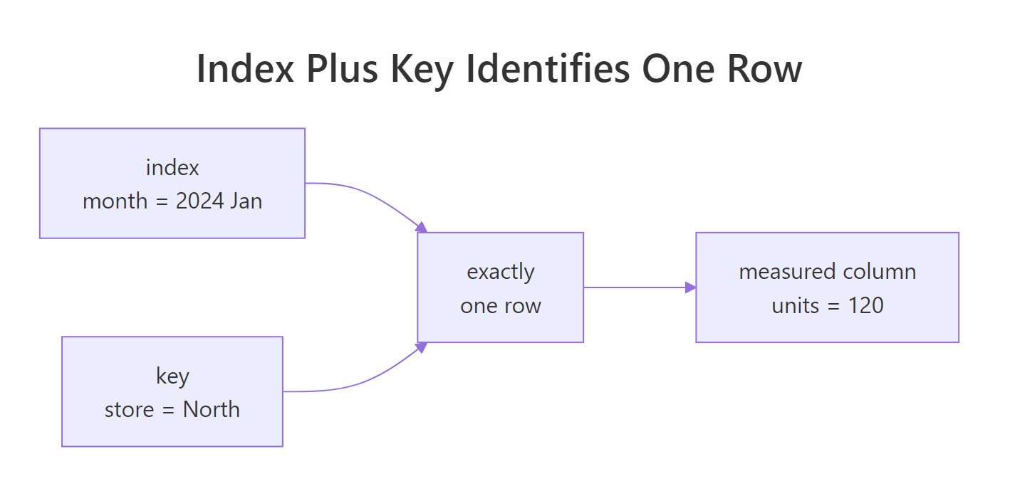
Figure 1: The index and the key together pick out exactly one row, and everything else is a measured value.
Two helper functions report what tsibble knows about your key.
n_keys() counts the series: 2, one per store. key_data() goes further and shows which rows belong to which series. The .rows column says North occupies 6 rows and South occupies 6 rows. On a table with 300 series, n_keys() is the fastest sanity check you have: if it returns 301 you have a typo somewhere in your identifier column.
The uniqueness promise is easy to verify by hand. Count how many rows share each month.
The as_tibble() step drops the tsibble structure for a moment so that count() behaves exactly as it would on any data frame, counting rows per month rather than per series. Each month appears twice, once for each store. That is allowed, because the combination of month and store is still unique. If any month appeared twice for the same store, tsibble would have refused to build the object at all, which is the subject of a later section.
Real tsibbles look exactly the same, just bigger. The pedestrian dataset ships with the tsibble package and records hourly foot traffic at four sensors in Melbourne.
Same structure, different scale. The index is Date_Time, the key is Sensor, the interval is [1h] (hourly), and there are 4 series sharing the 66,037 rows. The extra bit in angle brackets is the time zone, which tsibble tracks so that daylight-saving shifts do not quietly corrupt your hourly counts.
regular = FALSE to as_tsibble() and the interval will print as [!] instead.Try it: Report how many series pedestrian holds and what its interval is, using the two helpers you just met.
Click to reveal solution
Explanation: Four sensors means four series. The 1h interval is what tells forecasting packages later that a daily cycle spans 24 observations and a weekly cycle spans 168.
How do you turn your own data into a tsibble?
There are three doors into a tsibble, and which one you use depends on what you already have.
| You have | Use | Example |
|---|---|---|
| A data frame or tibble with a time column | as_tsibble(df, index = , key = ) |
Your CSV import |
A classic ts object |
as_tsibble(x) |
AirPassengers, USAccDeaths |
| Nothing yet, typing values by hand | tsibble(col = , ..., index = ) |
Small examples and tests |
Before any of them works, your time column has to be a real time type. R's built-in Date and POSIXct cover days and timestamps, and tsibble adds four classes for the coarser granularities.
| Granularity | Class to use | How to create it |
|---|---|---|
| Yearly | integer | 2024L |
| Quarterly | yearquarter |
yearquarter("2023 Q1") |
| Monthly | yearmonth |
yearmonth("2024-01") |
| Weekly | yearweek |
yearweek("2024 W01") |
| Daily | Date |
as.Date("2024-03-01") |
| Sub-daily | POSIXct |
as.POSIXct("2024-03-01 09:00") |
Start with the easiest door. A classic ts object already carries its own time information, so tsibble can read it without any help from you.
No index or key argument was needed. AirPassengers is monthly data from 1949, and as_tsibble() read the frequency straight out of the ts object, converted the timestamps to yearmonth values, and named the two resulting columns index and value. A single ts object holds only one series, so there is no key.
The second door is building a tsibble by hand, which is what you want for small examples.
tsibble() takes named vectors the same way data.frame() does, and the index argument names which of them is time. The [1Q] interval confirms it understood quarterly spacing, and <qtr> in the column header confirms the type.
The third door is the one you will use most: an ordinary table where the dates arrived as text.
as.Date() parses "2024-03-01" into a real date, then as_tsibble() detects that consecutive dates are one day apart and stamps the object [1D]. Skip the as.Date() step and as_tsibble() stops you immediately with Unsupported index type: character, which is the single most common first error people hit.
Now for the trap that catches almost everyone with monthly data.
This is monthly data stored as the first day of each month, which is how nearly every database exports it. But the values are Date objects, and the gaps between them are 31 and 29 days, so the largest step that divides both evenly is one day. tsibble concludes the data is daily, stamps it [1D], and then reports gaps: of the 61 calendar days between 1 January and 1 March, only 3 have rows, so 58 daily observations look missing. Nothing is broken, it just answered the question you accidentally asked.
Try it: Convert the built-in USAccDeaths time series (monthly US accidental deaths) into a tsibble and check its interval in the printed header.
Click to reveal solution
Explanation: 72 rows is six years of monthly observations, and the [1M] interval was carried over from the ts object's frequency of 12. Because it came from a ts, the columns are named index and value rather than anything descriptive. Rename them with rename() if you plan to keep the object around.
Why does as_tsibble() reject your data, and how do you fix it?
At some point as_tsibble() will refuse to build your object. This is the error, and it is worth reading carefully because it is telling you something true about your data.
Here is what happens if we forget the key on the two-store sales table.
The tryCatch() wrapper is only there so the page keeps running after the error; in your own console you would just see the message in red. What it means is simple. We claimed month alone identifies each row, but January appears twice, once for North and once for South. tsibble cannot honour the uniqueness promise, so it refuses.
The error message names its own debugging tool, so use it.
is_duplicated() answers yes or no, and duplicates() hands back every row caught in a clash so you can look at them. All twelve rows qualify here, so arrange(month) sorts them into pairs and head(4) shows the first two pairs. The answer is then plain to see: the two January rows carry the same timestamp and differ only by store, which is exactly the column we failed to name as the key.
That points to the two fixes, and choosing between them is a modelling decision, not a technical one.
Fix 1, name the missing key. If North and South really are two series you want to forecast separately, add key = store and you are done. That is what the very first code block did.
Fix 2, aggregate the duplicates away. If you only care about company-wide sales, collapse the two stores into one number per month first.
summarise(.by = month) adds up both stores for each month, leaving one row per month. Now month genuinely is unique, as_tsibble() accepts it, and you have a single national series. January's 218 is North's 120 plus South's 98.
Try it: A sensor logged two readings on 2024-05-02 by mistake. Use duplicates() to pull out just the offending rows.
Click to reveal solution
Explanation: duplicates() returns every row involved in a clash, not just the extras, so you can compare 22.8 against 23.1 and decide which to keep. With no obvious key column here, the honest fixes are to average the pair or to keep whichever reading the logger marked as valid.
How do you find the gaps hiding in a time series?
Here is the problem tsibble solves that a plain data frame cannot.
There are two ways a value can be missing from a time series. The first is explicit: the row exists, and the value in it is NA. You can see it, sum(is.na(x)) counts it, and every R function knows how to complain about it.
The second is implicit: the row is simply not there. March never made it into the export. There is no NA to find, because there is no row to hold one. Your data frame has 10 rows instead of 12 and looks completely healthy.
Implicit missingness is dangerous precisely because it is invisible. A forecasting model that assumes evenly spaced observations will treat February as if it were followed by May, and return a wrong answer without any warning or error.
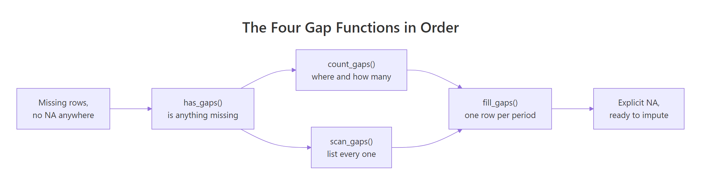
Figure 2: The four gap functions in the order you use them, from detection to explicit NA.
Let us break the sales data on purpose by deleting two of South's months, then ask tsibble whether anything is wrong.
The filter() call drops South's March and April, taking the table from 12 rows to 10. has_gaps() then reports one row per series with a .gaps flag: North is complete, South is not. That is the whole detection step, and on a table with 300 series it still returns one tidy row per series, so you can pipe it into filter(.gaps) to list the broken ones.
Knowing that South is broken is a start. Two more functions tell you where.
The two answer the same question at different zoom levels. scan_gaps() lists every missing timestamp individually, one row per hole, which is what you want when there are a handful. count_gaps() collapses consecutive holes into runs and reports the start (.from), the end (.to), and the length (.n), which is what you want when there are thousands.
On real data, count_gaps() is the one you reach for.
Eighteen separate outages across the four sensors, and the pattern in them is informative. Row 1 is a single missing hour on 5 April 2015, which is the night Melbourne's clocks went back for daylight saving. Rows 2 and 3 are 600 and 624 consecutive hours, roughly 25 and 26 days: the sensor was offline for most of May and most of October. Row 4 is a two-day outage. None of this is visible in the raw 66,037 rows, and none of it would produce a single NA.
Try it: Build a version of sales_ts where South's first three months are missing entirely, then compare has_gaps() with has_gaps(.full = TRUE). The two disagree, and the reason is worth knowing.
Click to reveal solution
Explanation: By default, every gap function judges each series against its own time span. South now runs from April to June with nothing missing inside that window, so the default answer is "no gaps". Setting .full = TRUE judges every series against the full span of the whole table, January to June, and then South's late start counts as three missing months. Use the default when series legitimately begin at different times (a store that opened in April), and .full = TRUE when every series is supposed to cover the same window.
How do you fill gaps so every period has a row?
Detection is half the job. fill_gaps() does the other half: it inserts the missing rows so the calendar is complete again.
South is back to six rows. March and April exist again, and their units values are NA. This is the crucial move: an invisible problem has become a visible one. Every R function that knows how to handle NA can now handle your data, and sum(is.na(sales_full$units)) finally returns 2.
You can also fill with a value instead of NA, by naming the column.
Whether that zero is right depends entirely on why the data is missing. If the store genuinely sold nothing in March, zero is the correct value. If the sales system was down, zero is simply wrong, and every model fitted to that history will forecast too low. Fill with zero only when absence really does mean none.
For most series, carrying the last known value forward is the safer default. fill_gaps() creates the rows and tidyr::fill() populates them.
March and April now hold 101, February's value, carried down. The group_by_key() call is what makes this safe: it tells fill() to work within each store separately, so North's last value can never leak into South's first gap. Without it, fill() would run straight down the combined table and do exactly that.
Try it: Fill South's two gaps with that store's own average instead of a fixed number. You will need group_by_key() for the average to be per-store.
Click to reveal solution
Explanation: With group_by_key(), mean(units) is evaluated inside each store, so South's gaps get South's average of its four observed months, 109.5, printed rounded as 110. Drop the group_by_key() line and mean(units) is computed across both stores instead, giving 128.2, which quietly imports North's larger numbers into South's series.
How does index_by() change the time granularity?
Hourly data is rarely the granularity you want to model. index_by() is the tool that moves between granularities, and it is best understood as group_by() for the time column only.
Here is hourly pedestrian traffic collapsed into daily totals per sensor.
Read the pipeline one step at a time. group_by_key() says "keep the four sensors apart". index_by(day = as_date(Date_Time)) creates a new index called day by throwing away the time-of-day part of each timestamp. summarise(daily_count = sum(Count)) then adds up the counts inside each sensor-day.
The result is still a tsibble, and its header proves the transformation worked: 66,037 hourly rows became 2,752 daily rows, the interval changed from [1h] to [1D], and the key survived with all 4 sensors intact. New Year's Day 2015 saw 8,950 people pass the Birrarung Marr sensor.
library(lubridate) a call to interval(sales_ts) will fail. Write tsibble::interval(sales_ts) to be explicit. This is a naming collision, not a bug in either package.The same pattern moves monthly data up to quarterly. When the new index is derived from the old one by a function, the tilde shorthand is tidier.
The ~ yearquarter(.) formula means "apply yearquarter() to the current index", with the dot standing in for whatever the index happens to be called. Twelve monthly rows became four quarterly rows, two per store. North's Q1 total of 394 is January's 120 plus February's 133 plus March's 141.
For simply cutting out a window of time rather than aggregating, filter_index() is a shortcut that saves you writing date comparisons.
The tilde reads as "from, to", and it is inclusive at both ends. It also understands partial dates, so "2015" means all of 2015 and "2015-03" means all of March 2015. The open forms . ~ "2024-04" and "2024-02" ~ . mean "everything up to" and "everything from".
Try it: Take the ped_daily object you just built and roll it up one more level, to monthly totals per sensor.
Click to reveal solution
Explanation: 2,752 daily rows became 95 monthly rows across four sensors. Notice May 2015 at 60,985 against March's 531,849: that is the 25-day outage count_gaps() found earlier showing up as a suspiciously small total. Aggregating over gaps sums whatever rows exist, so always fill gaps before you roll up, or a broken sensor will look like a quiet month.
Which dplyr verbs behave differently on a tsibble?
A tsibble is a data frame, so filter(), mutate(), select() and summarise() all work. Three of them behave slightly differently, and the differences trip people up until they know the rule: the index and key columns are structural, so tsibble protects them.
Start with select(), which is the most surprising.
We asked for one column and got three. That is deliberate. Dropping month would leave an object claiming to be a time series with no time in it, so tsibble adds the index and key back automatically. They move to the end of the column order, which is your visual cue that they were re-attached rather than requested.
summarise() goes the other way: it removes the key.
Without group_by_key(), summarise() treats the whole table as one thing and adds North and South together for each month, returning a single national series with no Key: line. That is either exactly what you wanted or a silent bug, depending on your intent. If you meant to keep the stores apart, group_by_key() before summarising is the fix, which is what the index_by() examples did.
For per-series calculations that keep every row, combine group_by_key() with mutate().
cumsum() restarts at each store rather than running continuously through the table, because group_by_key() scoped it. The as_tibble() at the end is the escape hatch: it strips the tsibble structure and hands back a plain tibble, which is what you want when you are done with time-series operations and just need a table to print or join.
Try it: Add a three-month rolling mean per store, computed with lag(). The first two months of each store have no history, so they should come out NA.
Click to reveal solution
Explanation: lag(units) reaches back one row and lag(units, 2) reaches back two, so March averages 120, 133 and 141 to get 131.3. January and February have nothing to reach back to, so the arithmetic yields NA. group_by_key() is what stops South's first month from lagging into North's last, which would silently produce a nonsense number instead of an honest NA.
Complete Example: from a messy raw table to a forecast
Time to put every step together on data that has both problems at once: a duplicated row and a stretch of missing months. This is what a real export from an orders database looks like.
First, build the raw table. Two regions, 24 months each, then one row accidentally duplicated and two months of West's data lost in transit.
Inside orders, the sin() term draws a gentle seasonal wave and rnorm() scatters random noise around it, so the numbers rise and fall the way real order volumes do. Forty-eight rows would be clean. We have 47, because one row was added and two were removed. The row count alone cannot tell you which rows were added and which were lost, and a plain data frame gives you no way to find out.
Step one is always to convert the time column and check for duplicates before doing anything else.
Passing both index and key to duplicates() asks the exact question as_tsibble() would ask, without triggering an error. The answer: East's May 2022 appears twice with identical values, a straightforward double-load.
Step two is to remove the duplicate and build the tsibble, then immediately ask about gaps.
summarise(.by = c(region, month)) puts every region-month combination into its own group, which is what gives as_tsibble() the one row per group it needs. The choice of summary function is where you have to think. Here the pair is one order batch that got loaded twice, so first(orders) keeps East's May at its real 221. Using sum() instead would have added 221 to itself and reported 442, inventing a month that never happened. In your own data, decide deliberately: sum() when the rows are separate real events that belong together, first() or max() when they are the same event logged twice.
The gap audit is unambiguous. East is complete; West is missing July and August 2022.
Step three is to repair the calendar and impute, per series.
Both regions now report FALSE. July and August carry June's 151 forward, and September resumes with its own real value of 132. The series is complete and evenly spaced, and because you ran count_gaps() first you know exactly which two values you invented.
Step four is the payoff. A complete keyed tsibble is exactly what the forecasting packages in the same family expect, so fitting a model to both regions at once takes one line.
model() read the key and fitted a separate seasonal naive model to each region. forecast(h = 3) produced three months ahead for each. Six forecast rows came back, two series by three horizons, and at no point did you write a loop or split the data.
That is the return on the setup work. Every step in this pipeline, from duplicates() to forecast(), was possible only because the object knew its own index, key and interval.
Practice Exercises
Exercise 1: Audit a device log
You have voltage readings from two devices over four days, except device B's log lost two of them. Build a keyed tsibble and report exactly which days are missing.
Click to reveal solution
Explanation: Six rows survive instead of eight, and the printed tsibble shows device B jumping straight from the 1st to the 4th. count_gaps() names the run: device B, 2 February through 3 February, two observations. Because both missing days sit inside B's own span, the default .full = FALSE is enough to catch them.
Exercise 2: Repair the log and prove it
Take the tsibble from Exercise 1, make the calendar complete, carry each device's last known voltage into its gaps, and then prove no gaps remain.
Click to reveal solution
Explanation: Six rows became eight, a complete four-by-two grid. Device B's 2nd and 3rd both carry 3.11 from the 1st, and device A is untouched because group_by_key() walled the two series off from each other. The final has_gaps() returning FALSE twice is the proof that the object is now safe to model.
Exercise 3: Find the busiest sensor-day in Melbourne
Using the ped_daily object built earlier, find the single sensor-day with the highest pedestrian count in the whole dataset.
Click to reveal solution
Explanation: 88,086 people passed the Birrarung Marr sensor on 8 March 2015, which was the Sunday of Melbourne's Moomba festival held in that exact park. The as_tibble() step matters: slice_max() reorders rows by value, and a tsibble warns when you break its temporal ordering. Dropping the structure first says "I am done treating this as a time series" and removes the warning entirely.
Frequently Asked Questions
Do I need a key if I only have one time series?
No. The key is optional, and a tsibble with no key is perfectly valid, as the annual profit and daily clicks examples showed. Add a key only when your table stacks two or more series on top of each other.
What is the real advantage over a plain ts object?
Three things. A ts object holds exactly one series, so 300 series means 300 objects or a wide matrix; a tsibble holds all 300 in one tidy table. A ts stores time as a start point plus a frequency, so it cannot represent an irregular or gapped series at all, whereas a tsibble stores real dates and can tell you precisely what is missing. And a tsibble is still a data frame, so every dplyr and ggplot2 skill you already have keeps working. The trade-off is that a lot of older forecasting code expects ts, which is why time series objects in R covers converting between all four classes.
Why does my interval say 1D when my data is monthly?
Because your dates are stored as Date values sitting on the first of each month. The gaps between them are 28 to 31 days, and the largest step that divides all of them evenly is one day. Convert the column with yearmonth() before calling as_tsibble() and the interval becomes 1M.
Can a tsibble hold irregularly spaced events?
Yes, with as_tsibble(regular = FALSE). The interval then prints as [!], and the gap functions no longer apply, since "missing" has no meaning when there is no expected spacing. Use it for event logs such as trades or clicks; use the regular form for anything you plan to forecast.
Does fable require a tsibble?
Yes. Every function in the fable and feasts packages takes a tsibble as input and reads the key to decide how many models to fit and the interval to decide the seasonal period. Getting the tsibble right is genuinely the prerequisite step, which is why the fable forecasting tutorial assumes the object already exists.
Summary
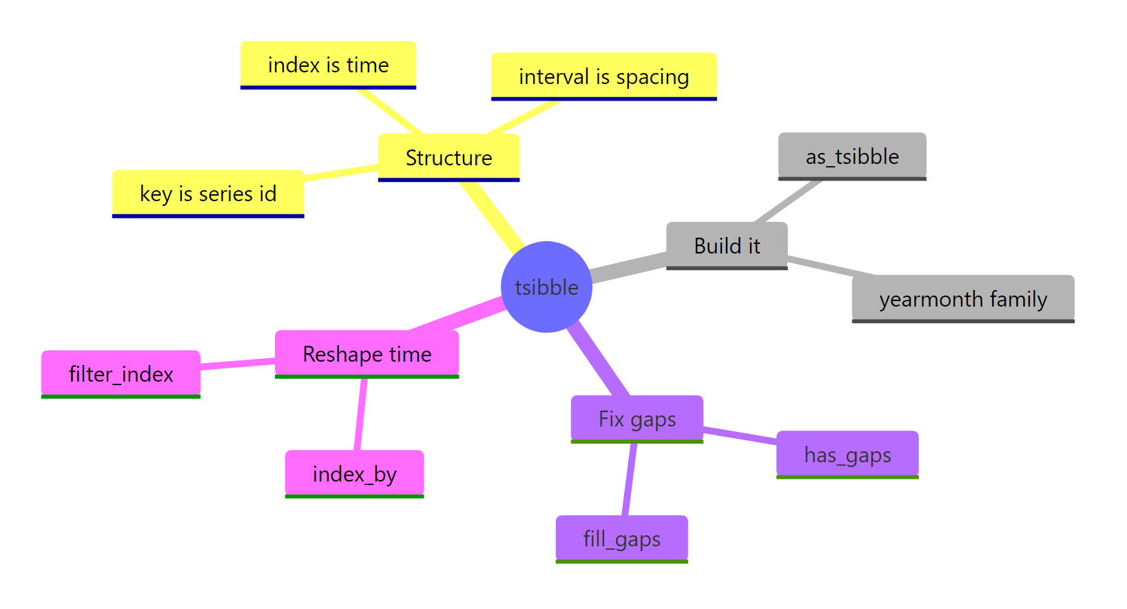
Figure 3: Everything tsibble gives you, grouped by the job it does.
| Job | Function | What it gives you |
|---|---|---|
| Promote a data frame | as_tsibble(index =, key =) |
A time-aware table |
| Build from scratch | tsibble(..., index =) |
Same, without a source frame |
| Convert coarse time | yearmonth(), yearquarter(), yearweek() |
The right interval instead of 1D |
| Inspect the contract | index_var(), key_vars(), interval(), n_keys() |
What the object thinks it is |
| Diagnose a build error | is_duplicated(), duplicates() |
The rows that broke uniqueness |
| Detect missing rows | has_gaps() |
One TRUE/FALSE per series |
| Locate missing rows | scan_gaps(), count_gaps() |
Every hole, or every run of holes |
| Repair the calendar | fill_gaps() |
Explicit NA rows you can impute |
| Change granularity | index_by() + summarise() |
Hourly to daily, monthly to quarterly |
| Cut a time window | filter_index("a" ~ "b") |
A slice without date arithmetic |
| Leave time behind | as_tibble() |
A plain tibble, no structure |
The three ideas worth carrying away:
- The index and key are a promise that each row is unique. When
as_tsibble()errors, it is telling you the promise is broken, and the fix is almost always naming a key column you forgot. - Implicit missingness is invisible until you look for it. A row that does not exist cannot be an
NA, so countingNAvalues proves nothing.has_gaps()is the only honest check. - Fix the calendar before you model. Duplicates, then gaps, then imputation, then aggregation. Doing it in that order means every later step operates on a complete, evenly spaced series.
References
- Wang, E., Cook, D., and Hyndman, R.J. "A New Tidy Data Structure to Support Exploration and Modeling of Temporal Data." Journal of Computational and Graphical Statistics, 29(3), 2020. Link
- tsibble package documentation. Link
- Introduction to tsibble (package vignette). Link
- Handle implicit missingness with tsibble (package vignette). Link
fill_gaps()reference page. Link- Hyndman, R.J. and Athanasopoulos, G. Forecasting: Principles and Practice, 3rd edition, Chapter 2: Time series graphics. Link
- Hyndman, R.J. "Tidy time series data using tsibbles." Link
- tidyverts, the tidy time series ecosystem. Link
- tsibble source repository on GitHub. Link
Continue Learning
- Forecasting with fable in R - now that you can build a clean tsibble, fit ETS, ARIMA and seasonal naive models to every series in it with a single
model()call. - Time Series Objects in R - how tsibble compares with
ts,zooandxts, and how to convert between all four when older code demands a different class. - Time Series Features in R - turn each series in a keyed tsibble into a single row of summary features, so you can triage hundreds of series at once.