VAR Models in R: Multivariate Time Series Forecasting

A VAR (vector autoregression) model forecasts several time series at once by letting every series depend on the recent past of every series in the system, including its own. In R you fit one with VAR() from the vars package, choose the lag order with VARselect(), and forecast with predict().

What is a VAR model, and when do you need one?

Employment and unemployment are two sides of one labour market. Each one carries information about where the other is heading, so a model that only looks at a series' own history throws half the evidence away. A VAR keeps both sides. The fastest way to see what that buys you is to fit one and ask it for a forecast.

We will work with Canada, a quarterly dataset that ships with the vars package. It holds four Canadian labour market indicators from 1980 to 2000. For now we take two of them: e (an index of employment) and U (the unemployment rate in percent).

Four lines of code produced a four-quarter forecast of the unemployment rate with prediction intervals. p = 2 tells VAR() to let each equation look two quarters back, and type = "const" says each equation gets its own intercept and nothing else (no trend term). In the output, the fcst column is the point forecast, lower and upper bound the 95% interval, and CI is the half-width of that interval.

Reading down the rows: unemployment is predicted to sit near 6.7% next quarter, and the interval widens from plus or minus 0.59 points to plus or minus 1.93 points by quarter four. Forecast uncertainty grows the further out you look, which a single point forecast would not have shown you.

The same fitted object also holds a forecast for employment, because a VAR models the whole system in one shot. That is the headline difference from ARIMA: one model, one estimation step, forecasts for every series you put in.

Here is the raw data those numbers came from.

Eighty-four quarters, four columns. The two columns we picked, e and U, move in opposite directions on the plot: when the employment index climbs, the unemployment rate falls. That mirror image is the relationship a VAR is built to exploit.

How does a VAR actually work under the hood?

A VAR looks intimidating written in matrix notation, so let us take it apart. With two variables and one lag, a VAR is just two ordinary regressions sitting side by side.

$$e_t = c_1 + a_{11} e_{t-1} + a_{12} U_{t-1} + \varepsilon_{1t}$$

$$U_t = c_2 + a_{21} e_{t-1} + a_{22} U_{t-1} + \varepsilon_{2t}$$

Where:

• $e_t$ and $U_t$ are employment and unemployment this quarter
• $e_{t-1}$ and $U_{t-1}$ are the same two variables one quarter ago
• $a_{11}$ is the effect of last quarter's employment on this quarter's employment, $a_{12}$ the effect of last quarter's unemployment on this quarter's employment, and so on
• $c_1, c_2$ are intercepts, and $\varepsilon_{1t}, \varepsilon_{2t}$ are the parts each equation cannot explain

Notice what the two equations have in common: the right-hand side is identical. Both regress on the same set of lagged variables. That is the defining property of a VAR, and it has a convenient consequence, which is that you can estimate each equation separately by ordinary least squares and get the same answer the full system would give.

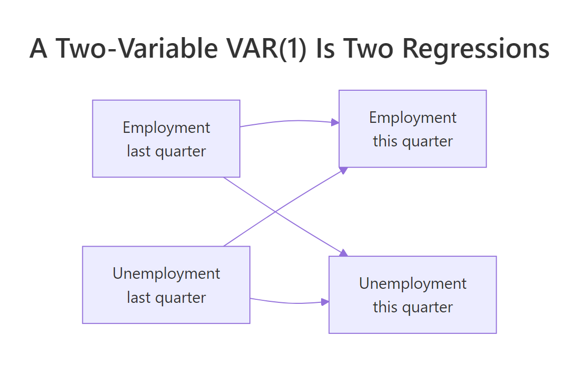
Figure 1: Every variable's past feeds every equation, which is what separates a VAR from two separate models.

Let us prove the claim rather than assert it. First we build the lagged dataset by hand: one column for each variable today, one column for each variable one quarter ago.

Row 1 pairs quarter two's values (e_now, U_now) with quarter one's values (e_lag1, U_lag1). Shifting the series by one row is all "lagging" means. We lose the first observation, since nothing precedes it, so 84 quarters become 83 usable rows.

Now fit the two equations with plain lm(), the same function you would use for any regression.

Two calls to lm(), six coefficients. The employment equation says employment is almost entirely explained by its own previous value (coefficient 1.0056), while last quarter's unemployment barely moves it (0.0097). Now watch what the vars package returns for the same specification.

Every number matches, digit for digit. Bcoef() returns the coefficient matrix with one row per equation, and row e holds exactly what lm(e_now ~ ...) produced. The package is doing the regressions you just did by hand, plus a lot of bookkeeping you would rather not write yourself.

Knowing the structure also lets you count parameters before you fit anything. With $K$ variables and $p$ lags, each equation has $Kp$ slopes plus an intercept, so the whole system estimates $K + pK^2$ coefficients. A 2-variable VAR(2) needs 10; a 5-variable VAR(4) needs 105, which is a lot to estimate from eighty-odd quarters.

Why must the series be stationary, and how do you check?

A series is stationary when its statistical behaviour does not depend on when you look at it: roughly constant average level, roughly constant spread, and a correlation structure that depends only on how far apart two points are. A series with a persistent upward drift is not stationary, because its average this decade differs from its average last decade.

This matters for a practical reason. Two unrelated series that both drift upward will look strongly related to a regression, purely because both happen to be going up. Econometricians call this a spurious regression, and a VAR fitted to drifting series is exposed to exactly that trap.

The standard check is the Augmented Dickey-Fuller test. Its null hypothesis is "this series has a unit root", which is the technical way of saying "this series is not stationary". A small p-value is therefore evidence for stationarity.

Both p-values sit far above 0.05, so neither test can reject the unit-root null. In plain terms, both series look non-stationary, which confirms what the plot showed. The model we fitted in section one was built on shaky ground.

The usual fix is differencing: instead of modelling the level of each series, model the change from one quarter to the next. diff() does this for every column of a multivariate series at once.

Row one now reads "employment rose by 0.193 index points and unemployment rose by 0.17 percentage points between 1980 Q1 and 1980 Q2". Differencing costs one observation, leaving 83 rows. Now retest.

Unemployment changes now pass the ADF test cleanly at 0.027. Employment changes come in at 0.083, which is suggestive but not decisive at the 5% level, so we bring in a second opinion. The KPSS test flips the hypotheses around: its null is "this series is stationary", so a large p-value is the reassuring one.

KPSS returns 0.1 for both series, which is the top of its reported range, so it fails to reject stationarity in either case. When ADF is borderline and KPSS is comfortable, the honest reading is that one round of differencing did the job and the ADF result reflects the low power of that test on 83 observations. We proceed with d_ec.

How do you choose the lag order p?

The lag order p answers one question: how far back should each equation look? Too few lags and the model misses real dynamics, leaving structure in the residuals. Too many and you burn degrees of freedom estimating coefficients that are mostly noise, which makes forecasts worse even though the in-sample fit improves.

Information criteria automate that trade-off. Each one scores a model on fit and then subtracts a penalty for the number of coefficients. VARselect() fits every VAR from 1 lag up to lag.max and reports which order each criterion prefers.

The four criteria split two against two. AIC and FPE want two lags; HQ and SC want one. That is normal, and the reason is their different penalties: SC (the Schwarz criterion, also called BIC) charges the most per coefficient and therefore picks the smallest models, while AIC is the most permissive.

The full scoreboard shows how close the race was.

Lower is better for every row. Reading the AIC row, lag 2 scores -4.8965 against lag 1's -4.8907, a margin so thin it would not survive a slightly different sample. All four criteria agree that anything past lag 2 is clearly worse, which is the more useful signal here.

How do you read and check a fitted VAR?

Now we fit the model we will keep: two variables, two lags, differenced data, with an intercept.

This table is the employment-change equation. Every coefficient answers the same shaped question: holding the other predictors fixed, how much does this quarter's change in employment move when that predictor moves by one unit?

The e.l1 coefficient of 0.9303 says a one-point rise in employment last quarter is associated with a further 0.93-point rise this quarter, so growth carries forward. The e.l2 coefficient of -0.5342 partly undoes it two quarters later, which is the signature of a series that overshoots and pulls back. Neither unemployment term reaches significance, so unemployment adds little to forecasting employment.

The unemployment equation is where the cross-series effect actually shows up.

Here the dominant term is e.l1 at -0.5871, with a t value of -4.40 and a p-value below 0.0001. Last quarter's employment growth predicts this quarter's fall in unemployment, and it does so far more reliably than unemployment's own history does.

Before trusting any of this, check that the system is stable. A VAR is stable when a one-off disturbance fades away as you run the equations forward, rather than growing without limit. roots() measures that for you: it rewrites the VAR as a single one-lag system (the companion form) and returns one number per variable per lag, each measuring how strongly the system carries a value forward one step. Every number must be below 1. A 2-variable VAR(2) therefore returns four numbers.

All four values sit near 0.47 and 0.33, comfortably below 1, so the model is stable and its forecasts settle down instead of growing. The adjusted R-squared values say the model explains 57% of the variation in employment changes and 43.5% in unemployment changes, which is respectable for differenced macro data.

The last checks look at the residuals, the part the model failed to explain. Well-behaved residuals show no correlation from one quarter to the next, hold a steady variance throughout, and follow a roughly normal distribution.

Each of these tests has "the residuals are well behaved" as its null hypothesis, so here a large p-value is the good outcome. The Portmanteau test returns 0.6433, meaning no leftover autocorrelation, which is the most important box to tick because it validates the lag choice. Normality passes comfortably at 0.8548.

The ARCH test fails at 0.0386. That flags volatility clustering: quiet quarters cluster together and turbulent quarters cluster together, which is extremely common in economic data.

Does one series really help predict another?

The coefficient tables hinted that employment predicts unemployment but not the reverse. Granger causality turns that hint into a formal test. The question it asks is precise: does adding the past of series X improve the forecast of series Y, beyond what Y's own past already provides?

The test works by comparing two nested models, one with X's lags and one without, using an F test. The null hypothesis is that all of X's lag coefficients in Y's equation are zero, so a small p-value means X does help.

The F statistic of 9.732 gives a p-value of 0.0001054, so we reject the null decisively. Employment history genuinely improves unemployment forecasts. Now the other direction.

A p-value of 0.2139 gives no reason to reject the null. Unemployment's past adds nothing measurable to the employment forecast once employment's own past is in the model. The influence in this system runs one way.

There is a second flavour of causality worth knowing. Granger causality is about lagged effects; instantaneous causality asks whether the two residuals are correlated within the same quarter.

The p-value of 0.000000152 is emphatic: the two shocks move together within a quarter. That makes sense, since a plant closing lowers employment and raises unemployment in the same three months, faster than quarterly data can separate. Remember this result, because it is exactly what forces the awkward assumption in the next section.

What happens to the whole system after a shock?

Coefficients tell you about one step. An impulse response function tells you about the whole chain reaction, and it is the single most useful output a VAR produces.

Picture the system sitting perfectly still, every variable at its long-run average. Now give one variable a single unexpected push, then leave the system alone and let its own equations run forward. The path that each variable traces out is the impulse response. The size of the push is one standard deviation of that variable's residuals, so "a one-standard-deviation employment shock" means a surprise about as large as the typical quarter-to-quarter surprise this model failed to predict.

The mechanics are simple to follow. A push to employment changes this quarter's employment. Next quarter, the equations feed that change into both variables through the lag terms. The quarter after that, those new values feed forward again, and because the model is stable the ripple shrinks each round until it disappears.

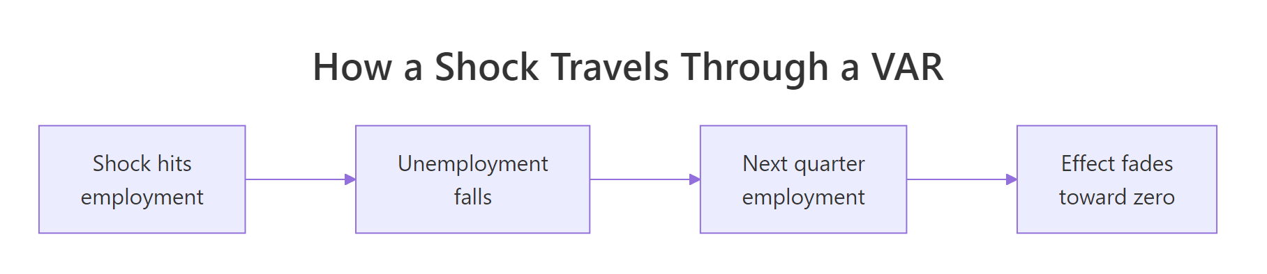
Figure 2: A shock enters one variable, spreads through the system, and fades.

Let us trace an employment shock through to unemployment.

Row 1 is the impact quarter and each row after it steps one quarter further ahead, out to eight. An unexpected burst of employment growth pushes the change in unemployment down by 0.237 percentage points immediately, holds nearly that full effect for another quarter, then decays through 0.164 and 0.081 until it is indistinguishable from zero by quarter five.

That decay pattern is the practical answer to "how long does a labour market shock last here?" About four to five quarters, on this data.

Point estimates alone can mislead, so the standard practice is to bootstrap a confidence band around them. Resampling the residuals many times produces many alternative impulse responses, and the spread of those tells you which part of the path is real.

The plot draws the response as a solid line with dashed bootstrap bands. Where the band stays entirely below zero, the effect is statistically distinguishable from nothing; where the band straddles zero, the apparent movement could be noise. On this model the band clears zero for the first few quarters and then closes around it, matching the decay you read off the numbers.

Now the caveat that separates careful VAR work from careless VAR work. Look at what happens when we send the shock the other way.

The impact response is exactly 0.0000. Not approximately zero, exactly zero, and no amount of data would change it. That zero was assumed, not estimated.

Here is why. We proved a moment ago that the two shocks are correlated within a quarter, so "shock employment while holding unemployment fixed" is not something the data can define on its own. To get a unique answer, irf() applies a Cholesky decomposition, which imposes a recursive ordering: the first variable in the system can affect the second on impact, but not the reverse. Since e comes first in our matrix, U is forbidden from moving e contemporaneously.

The companion tool answers a related question: not "what path does a shock trace" but "who is responsible for our forecast errors". Forecast error variance decomposition splits the uncertainty at each horizon into shares owned by each shock.

Each row is a forecast horizon and each column is a source of shocks; the row sums to 1. One quarter ahead, 51.6% of the uncertainty about unemployment traces back to employment shocks and 48.4% to unemployment's own shocks. By four quarters ahead the employment share has risen to 72.1% and settles there.

Put plainly: if you want to forecast Canadian unemployment more than a year out, most of what you do not know is really about employment. That is a concrete argument for keeping both series in the model.

How do you forecast, and does the VAR beat univariate models?

Forecasting from a fitted VAR is one function call. predict() runs the equations forward, feeding each quarter's predictions back in as the next quarter's lags.

Remember these are forecasts of changes, because we differenced. The model expects unemployment to fall by 0.224 points next quarter, with the expected change shrinking toward zero after that. The influence of the last observed quarters decays as the horizon grows, so far-out forecasts settle at the average change, which for a differenced series is close to zero. The fanchart() call draws the same information as shaded bands that darken toward the centre.

Forecasts of changes are hard to judge by eye, so the backtest below converts them back into levels before scoring them.

Whether the second series actually earns its place is a question the fitted output cannot answer. The honest test is to hide the last two years from the model, forecast them, and compare against what actually happened.

Two functions do the splitting. time() returns the calendar position of every observation in a quarterly series (1980.00, 1980.25, and so on), and window() cuts a slice out of a series using those positions, so train_lev stops at the eighth-from-last quarter and test_lev starts one quarter later. That leaves seventy-six quarters to learn from and eight to be judged on. The test window covers 1999 Q1 through 2000 Q4, and the model never sees it. Now fit both contenders on the training data only: our VAR, and a separate auto.arima() for each series, which is the strongest univariate baseline available without hand-tuning.

The cumsum() step is the piece worth pausing on: the VAR forecasts changes, so adding those changes cumulatively onto the last training level rebuilds a forecast of the level itself, which is what we compare against reality.

The VAR wins on both series. Root mean squared error for employment is 1.325 against ARIMA's 2.029, a 35% reduction, and for unemployment 0.882 against 1.479, a 40% reduction. On this holdout, the information each series carried about the other measurably improved both forecasts.

Seeing the paths side by side shows where the difference came from.

Unemployment actually fell from 7.90 to 6.87 over those eight quarters. The ARIMA model extrapolated the recent upward drift it had learned and kept climbing to 8.92, ending more than two points above the truth. The VAR levelled off near 7.9, still too high but by a much smaller margin, because employment growth in the training data pulled its unemployment forecast down.

Complete Example: the full four-variable Canada system

Everything so far used two series. Here is the same workflow applied to all four columns of Canada, start to finish, which is what a real analysis looks like.

All four differenced series test at or near the stationarity threshold, and the criteria repeat the two-against-two split we saw before. We take two lags again, which means estimating 4 + 2(16) = 36 coefficients from 81 usable rows, since differencing costs one quarter and the two lags cost two more.

A Portmanteau p-value of 0.9951 means there is essentially no autocorrelation left in the residuals, and the largest root of 0.6801 sits well inside the stability boundary. The model is sound enough to interpret.

Three of the four series Granger-cause the rest of the system: employment overwhelmingly, then productivity and real wages. Unemployment at 0.1547 is the odd one out, consistent with what the two-variable model told us, which is that unemployment is a follower rather than a leader in this data.

The forecast still points to unemployment falling for two quarters before flattening. The variance decomposition now spreads the credit across four sources: at a two-year horizon, employment shocks own 46.8% of unemployment's forecast uncertainty, real wages 15.5%, productivity 14.4%, and unemployment's own shocks the remaining 23.3%.

Frequently Asked Questions

When should I use a VECM instead of a VAR in differences? When your series are cointegrated, meaning they wander individually but never drift permanently apart. Differencing erases that long-run relationship, and a vector error correction model keeps it by adding a term that pulls the system back toward equilibrium. Test with the Johansen procedure, urca::ca.jo(), before differencing a set of series that theory says should move together.

How many variables can I put in a VAR? Fewer than you want to. A VAR estimates $K + pK^2$ coefficients, so going from 3 variables to 6 at two lags jumps from 21 coefficients to 78 while your sample size stays the same. With quarterly macro data most practitioners stop at three to six variables. Beyond that, look at Bayesian VARs or factor models, which shrink the coefficients toward zero instead of estimating each one freely.

Should I fit in levels or in differences? Differences are the safe default for non-stationary series, and that is what this tutorial used. Fitting in levels is defensible when the series are cointegrated, since the levels VAR remains consistent even though standard inference gets complicated. Fitting in levels because the tests were inconvenient is not defensible.

How is a VAR different from ARIMAX or dynamic regression? ARIMAX treats one series as the target and the others as external inputs, which means forecasting requires you to supply future values of those inputs. A VAR treats every series as both cause and effect, so it generates its own inputs and needs nothing from you. Use ARIMAX when the predictor is genuinely external, such as a published policy rate; use a VAR when the variables feed back into each other.

Why did my impulse responses change when I reordered the columns? Because orthogonalised impulse responses depend on the Cholesky ordering, which comes straight from your column order. Whichever variable is listed first is assumed to affect the others contemporaneously without being affected in return. Report the ordering you used, and check that your conclusions hold under a plausible alternative.

How do I add seasonal dummies or a deterministic trend? VAR() takes a season argument for centred seasonal dummies (season = 4 for quarterly data) and a type argument that accepts "const", "trend", "both", or "none". Include seasonality when the raw data is not seasonally adjusted; the Canada series already are, which is why we did not need it.

Practice Exercises

Exercise 1: Build and validate a three-variable VAR

Fit a VAR on the first differences of e, U, and rw from Canada. Choose the lag order with VARselect() using lag.max = 8, fit with type = "const", then prove the model is usable by showing the Portmanteau p-value and the largest stability root. Store the fitted model as cap1_fit.

Exercise 2: Find what drives real wages

Using the four-variable full_fit from the Complete Example, report the forecast error variance decomposition for rw at horizon 8 and at horizon 1. Identify which shock dominates at each horizon, and explain why the impact row is so lopsided.

Exercise 3: Does a third variable improve the forecast?

Backtest two competing models on the last eight quarters of unemployment. Model A is a VAR on the differences of e and U; model B adds rw. Train both on everything before the final eight quarters, cumulate the differenced forecasts back into levels, and compare RMSE against the actual test values.

Summary

A VAR is a system of ordinary regressions in which every series is explained by the recent past of every series. That single idea produces forecasts, causality tests, shock analysis, and variance decompositions, all from one fitted object. The workflow below is the order to run them in.

Figure 3: The six steps of a VAR analysis, from stationarity test to backtest.

Here is every function this tutorial used, with the question it answers.

The takeaways worth carrying forward:

• Difference first, model second. Non-stationary series invite spurious relationships, and the ADF p-value points the opposite way to most tests: a large value is the warning, not the all-clear.
• Pick the lag order with VARselect(), then confirm with the residuals. When the criteria disagree, prefer the larger order and check that serial.test() finds no leftover autocorrelation.
• Granger causality is about forecasting, not mechanism. It tells you which series carries information first, which is genuinely useful and is not the same as knowing what causes what.
• Impulse responses depend on the column ordering. The Cholesky assumption is yours to defend, so state it and test whether your conclusions survive a different one.
• Backtest against a univariate baseline. In-sample fit always improves when you add series, so a holdout comparison is the only evidence that the extra variables actually help. On the eight-quarter holdout here the VAR cut forecast error by 35% to 40% against auto.arima(), though the exercise at four quarters shows a single window can go the other way.

References

1. Pfaff, B. - VAR, SVAR and SVEC Models: Implementation Within R Package vars. Journal of Statistical Software 27(4), 2008. Written by the package author, and the clearest account of what each vars function estimates and why. Link
2. Pfaff, B. - vars package reference manual on CRAN. The argument-by-argument reference for VAR(), irf(), fevd() and the diagnostic tests used above. Link
3. Hyndman, R.J. & Athanasopoulos, G. - Forecasting: Principles and Practice (2nd ed), Section 11.2: Vector autoregressions. A short, worked treatment that pairs a VAR with the forecast package tooling used in the backtest here. Link
4. Hyndman, R.J. & Athanasopoulos, G. - Forecasting: Principles and Practice (3rd ed), Section 12.3: Vector autoregressions. The updated edition of the same chapter, rewritten around the fable framework if you prefer tidy syntax. Link
5. Lutkepohl, H. - New Introduction to Multiple Time Series Analysis. Springer (2005). The standard reference for VAR theory, including Cholesky identification and FEVD. Link
6. Trapletti, A. & Hornik, K. - tseries package reference, including adf.test and kpss.test. Link
7. Pfaff, B. - urca package reference, including the Johansen cointegration procedure. Link

Continue Learning

• ARIMA in R: What AR, I, and MA Mean and How to Fit One - the univariate foundation a VAR generalises, including what the AR terms in each VAR equation are doing.
• Test Stationarity in R - a deeper guide to the ADF and KPSS tests, including what to do when the two disagree.
• Dynamic Regression in R - the alternative approach for when one series is genuinely external rather than part of a feedback system.