Time Series EDA in R: Trend, Seasonality, Autocorrelation
Time series EDA is the set of checks you run before any forecasting: plot the series, measure its trend, detect its seasonality, split it into parts, then read the leftover autocorrelation to see what structure is still there. This guide runs that whole pass in R on real built-in datasets, one runnable step at a time.
Regular exploratory data analysis treats each row as a standalone observation. You compute a mean here, a histogram there, and the order of the rows does not matter. Time series data breaks that assumption completely. The rows arrive in a fixed order, and each value is tied to the one before it. That single fact, dependence over time, changes every question you ask of the data. This post walks the full EDA sequence for a time series in R, and you can run every block right here in the page.
What makes a time series different from ordinary data?
The honest starting point is that you cannot shuffle a time series. In a normal table you could reorder the rows and lose nothing. Reorder a time series and you destroy the very thing you came to study: how today depends on yesterday. So the first job of time series EDA is to put the data on a proper time axis and look at it. We will use base R for the structure and the forecast package for a few convenient plots.
Let's start with a series everyone can relate to: monthly totals of international airline passengers from 1949 to 1960. R stores it as a ts object, which is just a vector of numbers plus a calendar. Before plotting anything, it pays to ask three questions of that calendar: how often do observations arrive, when do they start, and how many are there?
The frequency is 12, which tells R that twelve observations make one natural cycle, a calendar year of months. The series starts in 1949 and holds 144 monthly readings. That frequency value is the single most important field in the object, because every seasonal tool below reads it to know how long one season lasts.
ts with the wrong frequency, decomposition and seasonal plots will look for a cycle of the wrong length and quietly return nonsense.Now the payoff. The first thing to do with any time series is plot it against time and simply look. The autoplot() function from forecast draws a clean time plot straight from a ts object.
Even this first glance answers a lot. The line climbs steadily from bottom-left to top-right, so there is an upward trend. It also wiggles up and down in a repeating pattern within each year, so there is seasonality. And the size of that yearly wiggle grows as the line rises. Hold on to that last observation, it decides a key choice later. Everything that follows is just measuring, one at a time, the things your eye already spotted here.
Try it: co2 is another built-in monthly series, atmospheric carbon dioxide measured at Mauna Loa. Find its measurement frequency and how many months it covers.
Click to reveal solution
Explanation: frequency() reports 12 because co2 is monthly, and length() counts 468 readings, which is 39 years of monthly data (39 times 12).
How do you spot and measure a trend?
A trend is the slow, long-run drift in the level of a series, ignoring the short-term wiggles. Your eye already saw the airline series climbing. The next step is to measure that climb instead of guessing at it. The simplest possible measure is the average value in each calendar year: if the yearly averages keep rising, you have an upward trend.
Here time(ap) gives the decimal year of every point (1949.0, 1949.083, and so on), floor() rounds each down to its whole year, and tapply() averages the twelve months inside each year. The averages rise from 127 up to 476, almost quadrupling over eleven years. That is the trend, now a number rather than an impression.
Yearly averages are blunt, though. They collapse a whole year into one point, so you lose all the detail in between. A moving average keeps the monthly resolution while still smoothing away the seasonal bounce. It slides a window along the series and replaces each point with the average of the window around it. Choose a window as wide as one full season, twelve months here, and each window contains exactly one of every month, so the seasonal ups and downs cancel out and the trend is left behind.
The ma(ap, order = 12) call computes the twelve-month moving average, and autolayer() draws it on top of the raw series. The jagged monthly line keeps its seasonal ups and downs, while the smooth line passes through the middle of them, tracing the underlying growth. That smooth line is your trend estimate at monthly resolution.
Try it: measure the trend in co2 the same way, by comparing the mean of its first full year (1959) to the mean of its last full year (1997).
Click to reveal solution
Explanation: window() cuts the series down to a date range, and averaging each year shows carbon dioxide rising from 315.8 to 363.8 parts per million, a clear upward trend.
How do you detect seasonality, and is it additive or multiplicative?
Seasonality is a pattern that repeats on a fixed calendar period: warmer summers every year, higher retail sales every December. The airline series has it, and the cleanest way to see the shape is to average each position within the season across all years. For monthly data, that means averaging all the Januarys, all the Februarys, and so on.
The cycle() function labels every observation with its position in the season, 1 through 12 for months, and tapply() averages within each label. The result is a clear seasonal fingerprint: travel dips in the winter months (February at 235) and peaks in July and August (both 351). That summer bump repeats every single year.
A picture makes the repetition obvious. A seasonal plot draws one line per year, all stacked on the same twelve-month axis, so you can see whether every year follows the same shape.
Every year's line has the same hump in the middle: the pattern is stable, only its size changes. And that change in size is the crucial detail. Look back at the raw plot, the summer peaks stretch further above the winter troughs as the years pass. When the seasonal swing grows with the level of the series, the seasonality is called multiplicative. When the swing stays the same size regardless of level, it is additive. We can settle the question by measuring the range (highest month minus lowest month) inside each year.
The within-year range widens from 44 in 1949 to 232 in 1960. The swing is not constant, it scales up with the level, so this seasonality is multiplicative. In symbols, an additive series and a multiplicative series decompose differently:
$$y_t = T_t + S_t + R_t \qquad\text{(additive)}$$
$$y_t = T_t \times S_t \times R_t \qquad\text{(multiplicative)}$$
Where $y_t$ is the observed value at time $t$, $T_t$ is the trend, $S_t$ is the seasonal component, and $R_t$ is the remainder. If formulas are not your thing, the practical point is all that matters: multiplicative means the parts multiply, so a percentage swing, not a fixed amount.
There is a simple trick that turns a multiplicative series into an additive one: take logarithms. Logs convert multiplication into addition, so a swing that grows in proportion to the level becomes a swing of constant size. We can confirm it by measuring the yearly range again on the logged series.
On the log scale the yearly range hovers around 0.4 the whole way through instead of growing. The swing is now roughly constant, which means the logged series is additive. That is why analysts so often model log(AirPassengers) rather than the raw counts: it lets them use the simpler additive machinery.
Try it: decide whether the seasonal swing in co2 is additive or multiplicative by checking its per-year range early, midway, and late.
Click to reveal solution
Explanation: The range creeps from 4.95 to 6.60 over 39 years, tiny growth against a level that sits near 315 to 360. The swing is essentially constant, so co2 is well described by an additive model.
How do you split a series into trend, seasonality, and noise?
So far you have measured the trend and the seasonality separately. Decomposition does both at once and hands you a third piece for free: the remainder, everything left after trend and season are removed. That leftover is where the real EDA payoff lives, as the next section shows. The diagram below is the mental model.
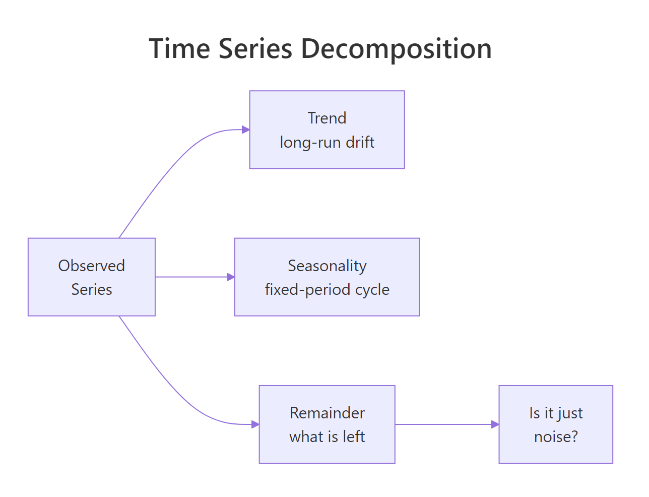
Figure 1: A time series splits into a trend, a seasonal cycle, and a remainder; EDA asks whether that remainder is just noise.
The classic tool is decompose(), which estimates the trend with a moving average, averages the detrended series by season to get a fixed seasonal pattern, and calls the rest the remainder. Because we found the airline series to be multiplicative, we ask for a multiplicative decomposition.
The dec$figure values are the twelve seasonal factors, one per month. Being multiplicative, they read as fractions of the trend: July and August sit at 1.227 and 1.220, meaning those months run about 22 percent above the yearly trend, while November at 0.801 runs about 20 percent below. This is the same summer-peaking story you saw earlier, now expressed as clean multipliers.
decompose() forces one fixed seasonal shape across the whole series. STL, in the stl() function, lets the seasonal pattern evolve slowly, handles any frequency, and is less affected by outliers. For most real series STL is the better default.STL (Seasonal and Trend decomposition using Loess) is the modern workhorse. It fits the trend and season with local regression, so both can bend over time. We run it on the logged series, lap, so the decomposition is additive and the components are easy to read.
The autoplot(fit) call stacks four panels: the data, then the trend, seasonal, and remainder that sum back to it. The printed table shows the first four rows of those three components on the log scale. Add the three numbers in any row and you recover that month's logged value. The seasonal column repeats every year, the trend column drifts upward slowly, and the remainder is the small leftover.
How strong are the trend and season, really? There is a tidy way to score each on a 0-to-1 scale. Compare the variance of the remainder alone to the variance of the remainder plus the component you care about. If adding the component barely changes the variance, the component is weak; if it dominates, the component is strong.
$$F_T = \max\!\left(0,\; 1 - \frac{\operatorname{Var}(R_t)}{\operatorname{Var}(T_t + R_t)}\right) \qquad F_S = \max\!\left(0,\; 1 - \frac{\operatorname{Var}(R_t)}{\operatorname{Var}(S_t + R_t)}\right)$$
Where $F_T$ is trend strength, $F_S$ is seasonal strength, and $T_t$, $S_t$, $R_t$ are the STL components. A value near 1 means that component explains almost all the variation; near 0 means it barely matters.
Both scores are close to 1: trend strength 0.994 and seasonal strength 0.937. This series is dominated by a very strong trend and a strong season, exactly what the plots suggested, now confirmed with a single pair of numbers you can compare across series.
Try it: decompose co2 with STL and compute its trend and seasonal strength.
Click to reveal solution
Explanation: co2 has an almost perfect trend (1.000) and a very strong season (0.984), which matches the steadily rising, cleanly cyclical shape of the Mauna Loa record.
What is autocorrelation, and how do you read an ACF plot?
Autocorrelation is the correlation of a series with a delayed copy of itself. Slide the series back by one step and correlate it with the original, and you get the lag-1 autocorrelation: how much this month resembles last month. Do it for lag 2, lag 3, and onward, and you get the autocorrelation function, or ACF. The formula is an ordinary correlation applied to the series and its own past:
$$r_k = \frac{\sum_{t=k+1}^{T} (y_t - \bar{y})(y_{t-k} - \bar{y})}{\sum_{t=1}^{T} (y_t - \bar{y})^2}$$
Where $r_k$ is the autocorrelation at lag $k$, $y_t$ is the value at time $t$, $\bar{y}$ is the series mean, and $T$ is the number of observations. You never compute this by hand, acf() does it, but it helps to see that a lag is just a shift and an autocorrelation is just a correlation.
The first value is always 1 (a series is perfectly correlated with itself at lag 0). After that the autocorrelations start high at 0.948 and fade slowly, then curl back upward toward lag 12 (0.760). Those two features are diagnostic. A slow, gradual decay is the signature of a trend: because the series is drifting, any two nearby points are similar simply because both are near the current level. The rise back up toward lag 12 is the signature of seasonality: a value is extra similar to the value one full year earlier.
The plotted version makes the pattern easier to scan and adds a significance band.
The dashed blue lines are the band inside which an autocorrelation is indistinguishable from zero. Bars that poke outside the band are real correlation; bars inside it are noise. For the airline series almost every bar clears the band, because trend and season leave strong autocorrelation everywhere. To see the opposite case, compare against a series with no structure at all: pure random noise.
Apart from the mandatory 1.000 at lag 0, every autocorrelation is tiny and hovers around zero. This is what "no structure left" looks like in an ACF: small bars, no decay, no seasonal echo. That contrast is the whole point of the ACF as an EDA tool. A structured series shows big, patterned bars; a random one shows nothing.
Try it: read the first few autocorrelations of co2 and say what the pattern implies.
Click to reveal solution
Explanation: The autocorrelations barely fall, from 0.991 at lag 1 to 0.934 at lag 6. That extremely slow decay is the fingerprint of a dominant trend, exactly the near-perfect trend strength the decomposition reported for co2.
How do you check whether the leftover is just noise?
This is the finish line of a time series EDA. After you have described the trend and the season, the question is whether anything predictable remains. If the remainder is pure random noise, you have captured all the structure. If it is not, there is still signal a forecasting model could use. The formal version of "is this just noise?" is the Ljung-Box test. It looks at a batch of autocorrelations at once and asks whether they are jointly close enough to zero to be random. A high p-value (above 0.05) means yes, it is noise; a low p-value means no, structure remains.
Start with the white-noise series from the last section, which we know is structureless by construction. It should pass.
The p-value is 0.9249, far above 0.05, so the test cannot reject randomness. This is what "just noise" looks like on the test: a large p-value. Now run the same test on the remainder from our STL decomposition of the airline series. If the trend-and-season split captured everything, this remainder should also pass.
The p-value is essentially zero, so the remainder fails the white-noise test decisively. Even after stripping out a smooth trend and a repeating seasonal pattern, the leftover still has autocorrelation the simple decomposition did not catch. That is not a failure of your EDA, it is the most useful finding in it.
That leftover structure usually has a name: the series is non-stationary, meaning its statistical behaviour changes over time. Most forecasting methods want a stationary series first, and the standard fix is differencing, replacing each value with its change from the previous period. Two helper functions estimate how many differences you need: ndiffs() for ordinary differencing and nsdiffs() for seasonal differencing.
Both come back as 1: take one seasonal difference and one ordinary difference to flatten the airline series. We can confirm that this actually produces stationarity with the KPSS test, whose null hypothesis is that the series is stationary. A p-value below 0.05 rejects stationarity; a high p-value is consistent with it. Run it on the logged series and again after differencing.
The diff(diff(lap), lag = 12) line does both differences in one step: the inner diff(lap) replaces each month with its change from the previous month (the ordinary difference), and the outer diff(..., lag = 12) then replaces each of those with its change from twelve months earlier (the seasonal difference). Before differencing the p-value is 0.01, so KPSS rejects stationarity: the raw logged series drifts, as expected. After one ordinary and one seasonal difference the p-value climbs to 0.10, so the test can no longer reject stationarity. The differenced series is stable enough to model. R also prints a "p-value smaller/greater than printed p-value" note here, which is normal: it just means the statistic fell past the ends of the test's lookup table.
adf.test() in tseries) has a null of non-stationarity, the reverse of KPSS, and it always fits a trend term, so it tests trend-stationarity specifically. Running both and comparing verdicts is more reliable than trusting either one alone.Try it: run the white-noise test on the STL remainder of co2 (reuse ex_fit from the strength exercise). Is anything left to model?
Click to reveal solution
Explanation: Like the airline series, co2's remainder fails the white-noise test, so a simple trend-plus-season split leaves autocorrelation behind. That leftover is what a model such as ARIMA would go on to capture.
Practice Exercises
These combine several steps of the EDA pass on series you have not seen yet. Each uses its own variable names so it will not disturb the airline session above. Try each before opening the solution.
Exercise 1: Profile the seasonality of nottem
The built-in nottem series holds twenty years of monthly average air temperatures at Nottingham Castle. Find its warmest and coolest months from the monthly means, then decide whether its seasonal swing is additive or multiplicative by checking the per-year range in three different years.
Click to reveal solution
Explanation: July is warmest (61.9) and February coolest (39.2), a clean summer-peaking season. The per-year range wobbles between about 19 and 31 with no upward drift, so the swing is roughly constant and nottem is additive. That makes sense physically, temperatures do not swing by a larger number of degrees just because the average is slightly higher.
Exercise 2: Measure structure in a quarterly series
The UKgas series records quarterly UK gas consumption. Quarterly data has a different season length from monthly data, so start by confirming the frequency, then decompose the logged series with STL and score its trend and seasonal strength.
Click to reveal solution
Explanation: The frequency is 4 because the data is quarterly, so one season is four points, not twelve. Both strength scores are high (trend 0.935, season 0.845), telling you UKgas is driven by a strong upward trend and a strong winter-heating season, the same profile you would confirm by eye on a time plot.
Exercise 3: Close the loop on nottem
Run the full white-noise check on nottem: decompose it with STL, pull out the remainder, and test it with Ljung-Box. Decide whether a simple trend-and-season split leaves anything for a model to capture.
Click to reveal solution
Explanation: The p-value is 0.0000352, well below 0.05, so even the tidy Nottingham temperature series leaves autocorrelated structure in its remainder. Month-to-month weather persistence is real, so consecutive residuals are related, and a model could still improve on the plain decomposition.
Frequently asked questions about time series EDA
What is the difference between decompose() and stl()? decompose() estimates one fixed seasonal shape with a moving average and holds that shape constant across the whole series. stl() fits the trend and season with local regression, so the seasonal pattern can change slowly over time. It also works with any frequency and is less affected by outliers. Use stl() as your default and keep decompose() for a quick look at a short, stable series.
How do I decide between an additive and a multiplicative model? Check whether the size of the seasonal swing grows as the level of the series rises. Compute the within-year range (the largest month minus the smallest) for several years: if that range grows with the level, the series is multiplicative, and if it stays about constant, the series is additive. Taking logs of a multiplicative series turns it into an additive one.
Do I need to remove the trend before reading the ACF? Yes, whenever the ACF decays slowly across many lags. A strong trend inflates every autocorrelation at once, so the individual bars stop being meaningful until you difference or detrend the series and plot the ACF again. On a trend-free series the bars show the genuine short-lag structure.
What does a very small Ljung-Box p-value mean? A p-value below 0.05 says the values you tested still carry autocorrelation, so the series or its remainder is not white noise. At EDA time that is a useful finding, not a problem: it means a forecasting model still has predictable structure to capture. A large p-value means the leftover is indistinguishable from random noise.
Which R packages do I need for time series EDA? Base R already provides ts objects plus decompose(), stl(), acf(), and Box.test(). The forecast package adds the tidier plots used here (autoplot(), ggseasonplot(), ggAcf()) and helpers such as ma(), ndiffs(), and nsdiffs(). The tseries package supplies the KPSS and ADF stationarity tests.
Summary
A time series EDA is a short, repeatable pass. You plot the series, measure the trend, characterise the season, split the parts, then interrogate the leftover. The workflow below is the order to run it in, and the table maps each step to its R tool.

Figure 2: The EDA pass, from the first plot to the white-noise test.
| Step | Question it answers | R tool |
|---|---|---|
| Plot the series | What does it look like over time? | autoplot() |
| Spot the trend | Is the level drifting? | yearly means, ma() |
| Detect seasonality | Is there a fixed-period cycle, additive or multiplicative? | cycle(), ggseasonplot() |
| Decompose the parts | How big are trend and season? | decompose(), stl(), strength scores |
| Read the ACF | What autocorrelation is present? | acf(), ggAcf() |
| Test the leftover | Is the remainder just noise, and is it stationary? | Box.test(), ndiffs(), kpss.test() |
The single most important idea is the last one. Decomposition and the ACF describe what is there; the Ljung-Box test tells you what is left. When the remainder fails the white-noise test, as it did for every real series here, you have found the predictable structure that a forecasting model will turn into forecasts.
References
- Hyndman, R.J. & Athanasopoulos, G. Forecasting: Principles and Practice, 3rd edition. Chapter 3: Time series decomposition. Link
- Hyndman, R.J. & Athanasopoulos, G. Forecasting: Principles and Practice, 2nd edition. Chapter 2.8: Autocorrelation. Link
- Cleveland, R.B., Cleveland, W.S., McRae, J.E. & Terpenning, I. STL: A Seasonal-Trend Decomposition Procedure Based on Loess. Journal of Official Statistics, 6(1), 3-73 (1990). Link
- R Core Team.
stl()reference, R stats package. Link - R Core Team.
decompose()reference, R stats package. Link - Hyndman, R.J. et al.
forecast: Forecasting Functions for Time Series and Linear Models. CRAN. Link - Ljung, G.M. & Box, G.E.P. On a Measure of Lack of Fit in Time Series Models. Biometrika, 65(2), 297-303 (1978). Link
- Kwiatkowski, D., Phillips, P.C.B., Schmidt, P. & Shin, Y. Testing the null hypothesis of stationarity. Journal of Econometrics, 54, 159-178 (1992). Link90104-Y)
Continue Learning
- Visualize Time Series in R: autoplot(), Seasonal, Lag Plots - the parent guide to every diagnostic plot for time series, in more depth than the plots used here.
- ACF and PACF in R: How to Read the Plots for ARIMA Orders - the next step once the ACF shows structure, turning those plots into model orders.
- Moving Averages in R: Simple, Weighted, and Exponential - a closer look at the smoothing tool used to expose the trend in this post.