NNETAR Model in R: Neural Network Time Series Forecasting
An NNETAR model is a neural network that forecasts a time series from its own past values. It is the nonlinear cousin of an AR model: the same lagged inputs go in, but they pass through a small hidden layer of neurons before they come out as a forecast. The nnetar() function in the forecast package fits one in a single line and chooses the architecture for you. This post shows what the model is, what the numbers in its name mean, how the network turns past values into a forecast, how to tune it, and, honestly, when it loses to ARIMA and ETS.
What is an NNETAR model, and when should you use it?
The lynx series counts Canadian lynx trapped each year from 1821 to 1934. It rises and crashes on a roughly ten-year cycle, and the rises are steeper than the falls. That asymmetry is nonlinear, which is exactly the shape a straight-line rule built from past values cannot bend to. One line of code fits a neural network to it instead. Press Run on the block below.
Read that printout from the top. NNAR(8,4) is the model R chose on its own: it decided to feed in the last 8 years of lynx counts and pass them through 4 hidden neurons. The line below says a 8-4-1 network with 41 weights, which is the same thing spelled out as an architecture: 8 inputs, 4 hidden units, 1 output. And Average of 20 networks means R did not fit one network, it fitted twenty and averaged them. The last line, sigma^2, is the average squared error the fitted network makes on the very data it trained on, so treat it as a description of the fit and not as a measure of forecast quality. We will unpack every one of those numbers.
For now, notice what you did not have to do. You did not choose lags, you did not choose a hidden layer size, you did not scale the data, and you did not initialise any weights. nnetar() made all of those decisions from the series itself.
An AR(p) model predicts the next value as a weighted sum of the last p values, and that weighted sum is a straight line. An NNAR model uses the same p lagged inputs, but routes them through neurons that bend. That single change is the whole idea.
Now let's turn the fitted model into an actual forecast and look at it.
forecast(fit_lynx, h = 20) runs the network forward 20 years. autoplot() draws the history in black with the forecast continuing on the right, and fc_lynx$mean holds the forecast numbers themselves, which is what we printed.
Look at the shape of those six numbers: 3892, then 3155, then a collapse to 232, then a slow climb back. The model has learned the boom-and-crash cycle and is projecting the next crash. A linear AR model fitted to this series produces a much rounder, more symmetric wave, because a straight-line rule cannot make the fall steeper than the rise.
So when should you reach for it? Use nnetar() when the series is long (roughly 100 observations or more), when the dynamics look nonlinear, and when point accuracy matters more to you than being able to explain the model to a stakeholder. Skip it when the series is short, when it has a strong trend (the limitations section below shows exactly why this breaks), or when you need prediction intervals you would defend in a meeting.
Try it: Fit an automatic NNETAR model to a different built-in series, sunspot.year (yearly sunspot counts from 1700 to 1988), and print just its model name with $method. The starter below fits lynx again, so change the series.
Click to reveal solution
Explanation: For sunspots R picks 9 lagged inputs and 5 hidden neurons. Sunspots have a longer cycle than lynx (about 11 years), so the model reaches further back to see a full cycle.
What do p, P, and k mean in NNAR(p,P,k)[m]?
You have now seen two model names, NNAR(8,4) and NNAR(9,5). The general form has four slots, and each one answers a different question about the network.
| Symbol | Name | What it controls |
|---|---|---|
p |
non-seasonal lags | How many recent values feed the network: lags 1 through p |
P |
seasonal lags | How many seasonal values feed it: lags m, 2m, up to Pm |
k |
hidden nodes | How many neurons sit in the hidden layer |
m |
season length | Observations per cycle, 12 for monthly, 4 for quarterly |
For a series with no seasonality, P and m are dropped and the short form NNAR(p,k) is used. So NNAR(8,4) means 8 lagged inputs and 4 hidden nodes, which is exactly the 8-4-1 architecture the printout reported.
Here is where those two numbers came from. When you do not supply p, nnetar() quietly fits a plain linear AR model first and lets AIC pick its order. AIC is a model-selection score that rewards a close fit but charges a penalty for every extra lag, so the order it picks is the smallest one that still explains the series well. Whatever order that search lands on becomes the network's lag count. Let's check that claim directly.
fit_lynx$lags lists the actual input lags, years 1 through 8 back. fit_lynx$size is the hidden layer width. And ar(lynx)$order is the AIC-optimal order of a linear AR model on the same series, which returns 8. That is not a coincidence: it is the rule.
The hidden layer size follows a formula. R sets $k = (p + P + 1)/2$, rounded. For lynx that is $(8 + 0 + 1)/2 = 4.5$, and R rounds a trailing .5 to the nearest even number, which gives 4 rather than 5.
Seasonal series get one extra ingredient. Let's fit AirPassengers, the classic 144-month record of international airline passengers from 1949 to 1960, counted in thousands. The call below carries one new argument, lambda = 0, which is unpacked in the note just after the printout.
Now the name has all four slots: NNAR(1,1,2)[12]. Decode it left to right. p = 1 means one recent lag, last month. P = 1 means one seasonal lag. k = 2 means two hidden neurons. [12] says the season is 12 observations long, which R read off the monthly series automatically.
So which two lags actually feed this network? Let's ask.
Lag 1 and lag 12. To predict next month, the network looks at last month and at the same month one year ago. That is a remarkably small model, just 9 weights, and the head-to-head comparison later shows it still forecasts respectably.
The weight count is also arithmetic, not magic. Every hidden node gets one weight per input plus a bias, and the output node gets one weight per hidden node plus a bias. For fit_air that is $(2 + 1) \times 2 + (2 + 1) \times 1 = 9$. For lynx it is $(8 + 1) \times 4 + (4 + 1) \times 1 = 41$, matching the printout exactly.
Try it: Fit AirPassengers with 3 non-seasonal lags instead of 1, keeping P = 1 and size = 2, then count the weights. Before you run it, work out the answer on paper: the inputs are lags 1, 2, 3 and 12, so 4 inputs.
Click to reveal solution
Explanation: Four inputs (lags 1, 2, 3 and 12) into 2 hidden nodes gives $(4 + 1) \times 2 = 10$ weights, plus $(2 + 1) \times 1 = 3$ for the output, so 13 in total.
How does the network actually turn past values into a number?
"Neural network" is usually where a tutorial stops explaining and starts calling it a black box. It does not have to be. A network this small is a handful of numbers and one curve, and in this section we are going to reproduce forecast()'s answer by hand with a calculator's worth of arithmetic.
To make that possible, let's deliberately build the smallest useful network. Two inputs feed a single hidden node, and we switch off the averaging so there is exactly one set of weights to look at.
A 2-1-1 network with 5 weights. That whole model, the thing that will produce a forecast, is five numbers. Let's look at them.
They come in a fixed order. The first three belong to the hidden node: a bias of 0.6772, then a weight of -2.2486 on lag 1 and 1.3845 on lag 2. The last two belong to the output: a bias of 2.1217 and a weight of -3.3008 on the hidden node's value.
A weight is the multiplier applied to one input, and a bias is a constant added on top no matter what the inputs are, exactly like the intercept in lm(). Every node in the network has one bias and one weight per incoming connection.
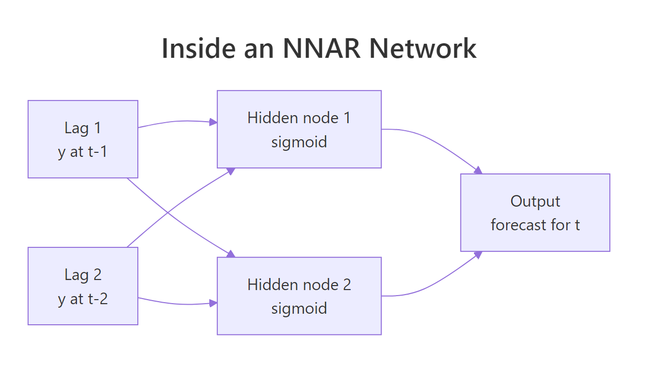
Figure 1: An NNAR(2,1) network: two lagged inputs, one hidden node, one forecast out.
Before the arithmetic, there is one preprocessing step to know about. By default nnetar() standardises its inputs, subtracting the mean of the series and dividing by its standard deviation, because neurons behave badly when fed raw values in the thousands. Those two numbers are stored on the model.
Now we have everything. The last two lynx observations are 2657 in 1933 and 3396 in 1934. To forecast 1935 the network takes lag 1 (3396) and lag 2 (2657), scales them, pushes them through the hidden node, and reads off the output.
If you would rather skip the equations, the code block after them does the same thing and you can jump straight there. Each hidden node computes a weighted sum of its inputs plus a bias, then squashes the result with the logistic sigmoid:
$$h = \sigma\left(b + \sum_{i=1}^{n} w_i x_i\right), \qquad \sigma(z) = \frac{1}{1 + e^{-z}}$$
Where:
- $h$ = the hidden node's output, always between 0 and 1
- $b$ = the hidden node's bias, 0.6772 here
- $w_i$ = the weight on input $i$
- $x_i$ = the scaled value of lag $i$
- $\sigma$ = the sigmoid, the curve that does all the bending
The output node then takes a plain weighted sum of the hidden values, with no sigmoid (that is what linear output units meant in the printout):
$$\hat{y}_{\text{scaled}} = b_o + \sum_{j=1}^{k} v_j h_j$$
Where $b_o$ is the output bias (2.1217), $v_j$ is the weight on hidden node $j$ (-3.3008), and $h_j$ is that node's value. Finally we undo the scaling with $\hat{y} = \hat{y}_{\text{scaled}} \times s + c$.
Let's run exactly that, one line per step.
Follow it through. Scaling turns 3396 into 1.1716 and 2657 into 0.7056, so both years were above the long-run average. The hidden node combines them into -0.9804. The sigmoid squashes that into 0.2728, a number between 0 and 1.
Now the last two steps: the output node, then undoing the scaling. Then we check the result against forecast().
3474.608 by hand against 3474.611 from forecast(). The gap of three thousandths is entirely because we rounded the weights to four decimal places before using them. Otherwise the numbers are the same, because they are the same calculation.
Try it: The sigmoid is the only nonlinear part of the whole model, so it is worth being able to compute it yourself. Change ex_h_in below to -0.9804 (the value our hidden node received) and check that the sigmoid returns 0.2728.
Click to reveal solution
Explanation: The sigmoid maps any real number into the range 0 to 1. It returns exactly 0.5 at an input of 0, drifts toward 0 for negative inputs and toward 1 for positive ones. Our input of -0.9804 sits below zero, so the output 0.2728 sits below 0.5.
Why does nnetar fit 20 networks and average them?
Every printout so far has said Average of 20 networks. That is the repeats argument, and its default of 20 exists for a specific reason: a neural network's answer depends on where its weights started.
Training begins from random weights and walks downhill until the error stops improving. But the error surface has many valleys, so a different random start can settle in a different valley and give you a different model. Let's make that visible by fitting single networks, twice, from different starting points.
Same function, same data, same settings. The only difference is the random seed, and the two models disagree completely. The first says lynx numbers keep climbing to 5515. The second says they crash to 1389. If you shipped either one as "the forecast", the number you shipped was decided by the random seed rather than by the data.
Now let's do exactly the same thing with the default of 20 networks averaged.
The two runs now tell the same story: a value near 4000, then a decline, then a further decline into the 1500 to 1800 range. They still are not identical, but the disagreement has shrunk from "crash versus boom" to a difference of a few hundred animals. Averaging cancels the luck of individual starting points.
There is a second thing worth understanding about these numbers. nnetar() trains the network to predict one step ahead, and nothing more. So how does it produce step 3?

Figure 2: Forecasts beyond step 1 are fed back in as inputs, so errors compound.
It feeds its own output back in. Step 1 uses real observations. Step 2 uses the step-1 forecast in place of the value it does not have yet. Step 3 uses steps 1 and 2. This is called recursive forecasting, and it explains why long-horizon neural network forecasts drift toward a flat line: after enough steps, the network is looking almost entirely at its own guesses.
set.seed() line immediately before every nnetar() call in anything you will rerun or hand to someone else.Try it: Confirm the seed rule for yourself. The starter uses two different seeds, so the check returns FALSE. Change the second seed to match the first and the two forecasts should become identical.
Click to reveal solution
Explanation: The seed fixes the random starting weights, so training follows the same path and lands on the same model. This is what makes a neural network forecast reproducible.
How do you forecast seasonal data with nnetar()?
We fitted fit_air earlier and found it uses just two inputs, lag 1 and lag 12. Now let's push it forward two years and see whether two inputs are enough to reproduce an annual travel pattern.
The plot shows the forecast picking up the series in 1961 and continuing the familiar sawtooth. The printed numbers say the same thing in figures: January 457, a dip in February to 436, then a steady climb into the summer peak, reaching 578 in June.
That shape is not something we told the model about. It emerged from the lag-12 input. Every time the network predicts a month, it is looking at what happened in that same month a year earlier, so February's dip and June's surge propagate forward on their own.
Note also that the forecasts sit above the historical values for those months, because the lag-1 input carries the series' upward drift into the first few predictions. The limitations section explains why that drift does not last as far as you might hope.
Try it: Fit a network to USAccDeaths, the monthly count of accidental deaths in the United States from 1973 to 1978, and read the season length off the model name. The starter fits lynx, which is yearly, so it has no seasonal slot at all.
Click to reveal solution
Explanation: The [12] comes straight from frequency(USAccDeaths), which is 12 because the data is monthly. R never asks you for the season length, it reads it from the ts object, which is why storing data as a proper ts matters.
How do you get prediction intervals from a neural network?
Every forecast so far has been a single line. Real forecasts need a range, and here NNETAR is genuinely different from ARIMA or ETS. Those models have a probability distribution built into their definition, so their intervals come from a formula. A neural network has no such distribution, so R has to simulate one.
The recipe is straightforward. Take the fitted network, forecast one step, add a randomly drawn error to it, feed that noisy value back in as a lag, and continue to the horizon. That gives one possible future. Do it a few hundred times and the spread of those futures is your prediction interval. Because that is real work, R does not do it unless you ask with PI = TRUE.
npaths = 200 is the number of simulated futures, kept modest here so the block runs quickly (the default is 1000, which is better for real work). Each row gives the point forecast plus four bounds. For January 1961, the model's best guess is 457.6 thousand passengers, it is 80% confident the truth lands between 425.8 and 485.3, and 95% confident it lands between 409.4 and 502.9.
Notice the intervals widening as you read down: January spans about 93 thousand at the 95% level, April spans about 98. That widening is the recursive feedback we saw earlier showing up as uncertainty. The further out you go, the more the network is forecasting from its own forecasts.
By default the simulated errors are drawn from a normal distribution. If your residuals are skewed or heavy-tailed, bootstrap = TRUE resamples actual historical residuals instead, which makes no distributional assumption.
Try it: Switch the error simulation from the normal default to bootstrapped residuals and compare the average width of the 95% interval. Add bootstrap = TRUE to the call below.
Click to reveal solution
Explanation: The average 95% interval widens slightly, from 103.1 to 104.1 thousand passengers. The two are close here because this model's residuals are already near-normal. On a series with occasional large shocks the bootstrap version would be noticeably wider, and more honest.
How do you tune nnetar with size, decay, and xreg?
The defaults are a reasonable starting point, not an answer. The argument that matters most is size, the number of hidden nodes, because it decides how much the model is able to memorise. Let's see what happens when we give it far too much capacity.
First we need an honest test. We hold back the last two years of AirPassengers so the model never sees them during training. window() is the base R function for cutting a ts object by date: end = c(1958, 12) keeps everything up to December 1958, and start = c(1959, 1) keeps everything after it.
141 weights fitted to 108 usable training rows. train holds 120 months, but with p = 12 the first 12 are consumed as lags for the thirteenth, so only 108 rows can actually be predicted. There are more parameters than data points, which should worry you. Let's score it on both sets and see whether it does.
accuracy() scores a forecast against the truth, and the three columns are the standard error measures. RMSE is the root mean squared error, the typical miss in passenger units with big misses weighted heavily. MAE is the mean absolute error, the typical miss with every miss weighted equally. MAPE is the mean absolute percentage error, the typical miss as a percentage of the actual value.
Read the two rows against each other. On data it trained on, the model is off by 2.13 thousand passengers on average, which looks superb. On data it has never seen, it is off by 69.29, more than thirty times worse. The model did not learn the pattern, it memorised the training years.
The fix is decay, which penalises large weights during training and so pushes the network toward simpler behaviour. Let's add it and change nothing else.
The training error got six times worse and the test error improved by a quarter. That trade is the entire point of regularisation: we gave up a fit we could not trust for a fit that generalises better.
sigma^2 on the printout and the training-set row of accuracy() both measure how well the network memorised its own training data, and a big enough network can drive both to nearly zero while forecasting terribly. The test-set row is the only number that answers your actual question.Try it: The oversized model above has 10 hidden nodes. Reduce size to 2 and see what the test RMSE does. Everything else stays the same.
Click to reveal solution
Explanation: Test RMSE drops from 69.29 to 42.98 just by removing hidden nodes. Shrinking the network beat adding regularisation to the large one (51.68), which is a common pattern: the cheapest fix for overfitting is usually a smaller model.
Can nnetar use external regressors with xreg?
Sometimes the series' own past is not the whole story. A promotion, a holiday, a price change, or a temperature reading can drive the value you are forecasting, and nnetar() accepts those as extra inputs through xreg. Each column of xreg simply becomes another input node alongside the lags.
To see the effect cleanly, let's build a series where we know an external driver matters, because we put it there. Monthly sales follow a seasonal wave, and in months with a promotion they jump by 25 units.
We made 132 months, kept the first 120 for training and held back the last 12 for testing. promo is a 0/1 indicator that is on about a quarter of the time. Notice that we also kept promo_future, the indicator values for the test months. You must have future values of any regressor to forecast with it, which is the practical catch with xreg.
Now fit the same series twice, once blind to the promotions and once told about them.
Both models chose the same NNAR(1,1,2)[12] shape, but the second has 11 weights instead of 9. Those two extra weights are the promotion input wiring into each of the two hidden nodes. Let's see whether they earn their keep.
Test RMSE more than halves, from 12.44 to 5.82. The blind model can only average over promotion and non-promotion months and land somewhere in between. The informed model knows which months get the 25-unit bump and moves its forecast accordingly.
Note the syntax difference in the second call: when a model was fitted with xreg, forecast() demands the future regressor values through xreg = as well. Forget it and R throws an error rather than guessing.
Try it: Confirm the input count directly rather than inferring it from the weights. nn_yes$model[[1]]$n holds the network's layer sizes as a vector of three numbers: inputs, hidden nodes, outputs.
Click to reveal solution
Explanation: The first column is the input count: 2 lags alone, versus 2 lags plus 1 regressor. The hidden layer (2) and output layer (1) are unchanged, which is why the weight count went up by exactly 2, one connection from the new input to each hidden node.
Does nnetar actually beat ARIMA and ETS?
Most tutorials on this topic never answer it. Neural networks sound more powerful than the classical methods, so it is easy to assume they forecast better. Let's just measure it, on the same train and test split we built while tuning.
Three automatic model selections, three different answers. The neural network chose a 9-weight NNAR(1,1,2)[12], auto.arima() chose the airline model, and ets() chose additive error, trend and seasonality. All three saw exactly the same 120 months of training data. Now we score them on the 24 months none of them saw.
Read the RMSE column. ETS wins at 26.54, the neural network is second at 37.33, and ARIMA comes last at 43.18. MAPE tells the same story: ETS is off by 4.47% on average, NNETAR by 5.59%, ARIMA by 8.52%.
So the honest answer is: sometimes, and not here. The neural network comfortably beat ARIMA on this series while using a fraction of the parameters, but a classical exponential smoothing model beat both. That is a very typical result. Neural networks earn their advantage on nonlinear dynamics, and monthly airline passengers are mostly trend plus seasonality, which is precisely what ETS was designed for.
tsCV(), which scores each model over many origins instead of one.Try it: Add a fourth contender, the seasonal naive forecast, which simply repeats last year's value for each month. If a model cannot beat that, it is not earning its complexity.
Click to reveal solution
The starter already runs the benchmark, so the exercise is reading it. Seasonal naive scores a test RMSE of 76.99, well behind all three fitted models.
Explanation: The neural network halves the naive error, so it is genuinely learning something. Always run this check. On a series with a weaker signal, a model that looks respectable in isolation can turn out to be no better than repeating last year.
What are nnetar's limitations, and how do you work around them?
Here are the five failure modes you will run into in practice, with the biggest one demonstrated in code.
| Limitation | Why it happens | What to do |
|---|---|---|
| Cannot extrapolate a trend | nnetar() never differences the series |
Difference it yourself, or use ARIMA or ETS |
| Needs a long history | Many weights, few observations | Prefer classical models under roughly 100 points |
| No interpretable coefficients | Weights have no individual meaning | Use ARIMA if you must explain the model |
| Optimistic prediction intervals | Simulation assumes the model is correct | Report them as a lower bound |
| Different answer every run | Random starting weights | Always set.seed(), keep repeats at 20 or more |
The trend problem is the one that surprises people, so let's watch it happen. This series is about as easy as forecasting gets: it starts at 50 and climbs by exactly 2 per period, with a little noise.
The series ends around 170 and should continue to roughly 190 over the next ten periods. Instead the forecast flattens at 166 and then edges slightly down. The model does not merely fail to project the trend, it reverses it.
The reason is not that the network is weak, it is that the trend takes the inputs somewhere the network has never been. Predicting period 61 requires an input around 170, which is at the very edge of the training range, and every step after that would need inputs beyond it. A sigmoid flattens out at both ends of its range, so once the inputs push past the training range it returns almost the same value for every one of them, and the forecast goes flat.
A model that does difference the series has no such problem. Same data, one line.
auto.arima() climbs from 170.1 to 189.0, almost exactly the true path. The difference is not intelligence, it is differencing: ARIMA models the period-to-period changes, which have no trend at all and so stay comfortably inside the range it was trained on.
That points straight at the fix. If you want a neural network on a trending series, difference it first, model the changes, then add them back up.
Three steps. diff() converts levels into changes. The network forecasts the changes, which hover around 2 and stay well inside the range it learned. Then cumsum() adds those changes onto the last observed value to rebuild levels.
The result climbs from 171.5 to 192.1, tracking the real trend. It is bumpier than the ARIMA path because the network is also modelling noise in the differences, but the systematic failure is gone.
ARIMA(0,1,1) tells you it worked on first differences. An NNAR name has no such slot, because there is no such step. Checking your series for trend before you fit is your job, not the function's.Try it: Compare the model that nnetar() chooses on the original trending series against the one it chooses on the differenced series. The two are already fitted above as nn_tr and nn_d.
Click to reveal solution
Explanation: On the raw trending series R picks NNAR(1,1), a single lag into a single neuron, because a trend is almost perfectly predicted by the previous value and nothing else adds much. After differencing, the trend is gone and the genuine short-run structure becomes visible, so R reaches for 4 lags and 2 neurons.
Complete Example: forecasting US accidental deaths
Let's run the whole workflow end to end on a series we have not modelled yet: USAccDeaths, monthly accidental deaths in the United States from 1973 to 1978. We will split the data, fit a network, benchmark it against something dumb, and only then decide what to ship.
Sixty months of training data, and R fits an NNAR(2,1,2)[12] with 11 weights: lags 1, 2 and 12 into two hidden nodes. That is a sensibly small model for a short series. Now the step most people skip.
The neural network loses. Repeating last year's figures beats it on every measure, with an RMSE of 341 against 547 and a MAPE of 2.85% against 5.33%.
This is a real result, and the reason matters. USAccDeaths is a strongly seasonal series with only 60 training months, which means the network sees each calendar month just five times. There is not enough history for it to learn the seasonal shape better than simply copying it, and the tuning grid below confirms that no hidden layer size rescues it.
Every size lands between 546 and 620, all worse than seasonal naive's 341. The right decision here is to ship snaive() for this series, or to try ETS, and to record that NNETAR was tested and rejected. A workflow that can return "no" is worth more than one that always returns a neural network.
For completeness, here is what shipping the network would have looked like: refit on all 72 months and forecast the next year with intervals.
Refitting on the full series before forecasting is standard practice: the split existed only to choose a model, so once chosen, the model should learn from every observation you have.

Figure 3: A safe nnetar workflow: split, seed, tune, score, then refit on everything.
Practice Exercises
These combine several ideas from the tutorial. They use variable names starting with my_ so they will not disturb anything fitted above.
Exercise 1: Find the best hidden layer size for AirPassengers
The default nnetar(train, lambda = 0) scored a test RMSE of 37.33 in the head-to-head comparison. Loop size from 1 to 6, refit each time on train with set.seed(88) inside the loop, score each on test at h = 24, and report which size wins.
Click to reveal solution
Explanation: Five hidden nodes wins with a test RMSE of 29.88, well ahead of the default's 37.33 and now close to the 26.54 that ETS managed. The curve falls to a minimum at 5 and rises again at 6, which is the overfitting from the tuning section starting to appear. Note that set.seed() goes inside the function so every candidate starts from the same random weights and the comparison is fair.
Exercise 2: Rescue the default model on lynx
The automatic choice for lynx was NNAR(8,4), 8 lags into 4 neurons. Test whether that is actually a good choice: train on lynx up to 1920, test on 1921 onward (14 years), and compare p values of 2, 4, 8 and 12 with set.seed(12). Use window() to build the split.
Click to reveal solution
Explanation: Two lags beat eight by a factor of four, 418.5 against 1682.9. The default p comes from an AIC fit on the training data, which rewards explaining the past rather than predicting the future. On a 14-year horizon the small model wins because its forecasts have far less room to compound their own errors. Never assume the automatic order is the best forecasting order.
Exercise 3: Write a reusable differenced-nnetar function
The limitations section showed the difference-then-undo trick as loose lines of code. Package it into a function nnetar_diff(y, h, seed) that differences the series, fits a network, forecasts h steps, and returns forecasts on the original scale. Test it on my_series, a trending series built the same way as trend_ts.
Click to reveal solution
Explanation: The function reproduces the earlier numbers exactly, which is the point: same recipe, now reusable. Taking seed as an argument keeps results reproducible while letting you check stability across seeds. One caveat to remember, the returned values are point forecasts only. Prediction intervals do not survive cumsum(), because summing the bounds of each step ignores how the errors accumulate.
Frequently Asked Questions
Is NNETAR a deep learning model like an LSTM? No. NNETAR has exactly one hidden layer and typically fewer than 50 weights, while an LSTM has many layers, a memory mechanism, and thousands of parameters. NNETAR is a small, fast, classical neural network aimed at series with a few hundred observations. On short business series that simplicity is usually an advantage rather than a compromise.
Why do I get different forecasts every time I run the same code? Training starts from random weights, so each run explores a different path. Put set.seed() immediately before every nnetar() call, and leave repeats at 20 or higher so the averaging smooths out whatever start you got.
How much data does nnetar need? As a rough rule, at least 100 observations, and for a seasonal series at least several full cycles so the network sees each seasonal position many times. The complete example above shows what happens with only 5 years of monthly data: the network loses to a naive benchmark.
Do I need to make the series stationary first? Not for seasonality, which the seasonal lag handles. But yes for trend, because nnetar() never differences. If your series trends, difference it yourself as shown in the limitations section, or use a model that differences for you.
Why is PI = TRUE so slow? Because it does not use a formula, it simulates. With the default npaths = 1000 R runs the whole recursive forecast a thousand times. Drop npaths while you are exploring, and raise it for the final run.
What is the difference between nnetar() and NNETAR() in fable? They fit the same model with the same defaults. nnetar() from forecast works on ts objects, while NNETAR() from fable works on tsibble objects inside a model() call. Pick whichever package the rest of your pipeline uses.
Can NNETAR handle multiple seasonal periods, like daily data with weekly and yearly cycles? Not directly. nnetar() reads a single frequency() from the series. For multiple seasonality, supply Fourier terms as xreg, or use a model built for it such as TBATS.
Summary
| Concept | What to remember |
|---|---|
| What it is | A feed-forward neural network fed lagged values of the series, a nonlinear AR model |
| Model name | NNAR(p,P,k)[m]: p recent lags, P seasonal lags, k hidden nodes, m season length |
| Defaults | p from an AIC-optimal linear AR fit, P = 1, k = (p+P+1)/2 rounded |
| Weight count | $(\text{inputs} + 1) \times k + (k + 1)$ |
repeats = 20 |
Fits 20 networks from random starts and averages them, cancelling the luck of initialisation |
| Reproducibility | set.seed() before every fit, or the forecast changes on every run |
| Multi-step forecasts | Built recursively by feeding each forecast back in, so errors compound with horizon |
| Prediction intervals | Need PI = TRUE, come from simulation, and are optimistically narrow |
| Tuning | size first, then decay to regularise; judge only on held-out data |
xreg |
Extra input nodes for external drivers; you must supply their future values |
| Biggest limitation | No differencing, so it cannot extrapolate a trend. Difference the series yourself |
| Honest expectation | Strong on nonlinear cyclical series, often beaten by ETS on trend-plus-season data |
References
- Hyndman, R.J. & Athanasopoulos, G. Forecasting: Principles and Practice, 3rd edition, Section 12.4: Neural network models. Link
- Hyndman, R.J. & Athanasopoulos, G. Forecasting: Principles and Practice, 2nd edition, Section 11.3: Neural network models. Link
- forecast package reference,
nnetar(): Neural Network Time Series Forecasts. Link - forecast package reference,
forecast.nnetar(): Forecasting using neural network models. Link - Hyndman, R.J. Prediction intervals for NNETAR models, Hyndsight blog. Link
- nnet package on CRAN, the feed-forward network engine
nnetar()calls. Link - forecast source code for
nnetar(), robjhyndman/forecast on GitHub. Link - fable package reference,
NNETAR()for tsibble workflows. Link
Continue Learning
- ARIMA Models in R walks through the model family that beat NNETAR on trending data, and explains the differencing step NNETAR lacks.
- ETS Models in R covers the exponential smoothing framework that won the head-to-head comparison in this post.
- Forecast Accuracy in R explains what RMSE, MAE and MAPE actually measure, and which one to trust when they disagree.
- Time Series Cross-Validation in R shows how to score models over many rolling origins instead of a single split, which is the right way to settle the NNETAR versus ETS question on your own data.