Distributional Forecasts in R with fable
A distributional forecast gives you a whole probability distribution for each future time point, not just a single best guess. In the fable package that distribution is the actual value stored in your forecast table, and the familiar point forecast is just one number summarised out of it. Once you see the table that way, prediction intervals, quantiles, simulated futures and forecast scores all stop being separate topics and become four questions you ask of one object.
What does forecast() actually hand back?
Most people run forecast(), glance at the point forecast column, and move on. That column is the least interesting thing in the table. Let us fit a model to Victorian department store sales and look carefully at what comes back.
The data is aus_retail, a set of Australian retail turnover series that ships with the tsibbledata package. We will pull out one series, department stores in Victoria, and hold back 2018 so we have real numbers to check ourselves against later.
Let us walk through what happened. summarise() collapsed the two key columns (State and Industry) down to a single series, filter_index() trimmed it to 2000 through 2018, and the split kept everything up to December 2017 for training. ETS() fitted an exponential smoothing model, which works out for itself whether the trend and the seasonal pattern should be added on or multiplied in. Then forecast(h = 12) asked it for the twelve months of 2018.
Now read the result carefully, because this is the whole point of the page. There are two columns of numbers, not one.
The Turnover column has type <dist>, and its first entry reads N(351, 222). That is not a formatted string. It is a normal distribution stored in a table cell, with a centre of 351 and a spread of 222. The .mean column next to it holds 351., which is simply the mean of that distribution, computed for your convenience.
So the model did not predict "351 million dollars of turnover in January". It predicted a bell curve centred on 351, and somebody rounded that bell curve down to its centre point to fill in .mean.
You can prove the distribution column is a real object by pulling a value out of it.
That confirms it. fc$Turnover is a vector of class distribution with twelve elements, one probability distribution per forecast month. It behaves like any other column: you can subset it or hand it to other functions.
And because each element is a genuine distribution, you can ask it the questions you would ask any distribution. Three of the four calls below are ordinary base R. variance() belongs to the distributional package, so it is written as distributional::variance(): the package::function() form calls a function straight out of a package without loading it first, which is convenient here because distributional is installed automatically alongside fable.
Four questions, four answers. The mean is 350.77 and the median is identical, which is what you expect from a symmetric bell curve. The variance is 221.9, and its square root, the standard deviation, is 14.9.
That last pair of numbers exposes a trap in the way the distribution column prints.
N(351, 222) and its standard deviation is sqrt(222), roughly 14.9, so an interval built by eyeballing "351 plus or minus 222" would be about fifteen times too wide.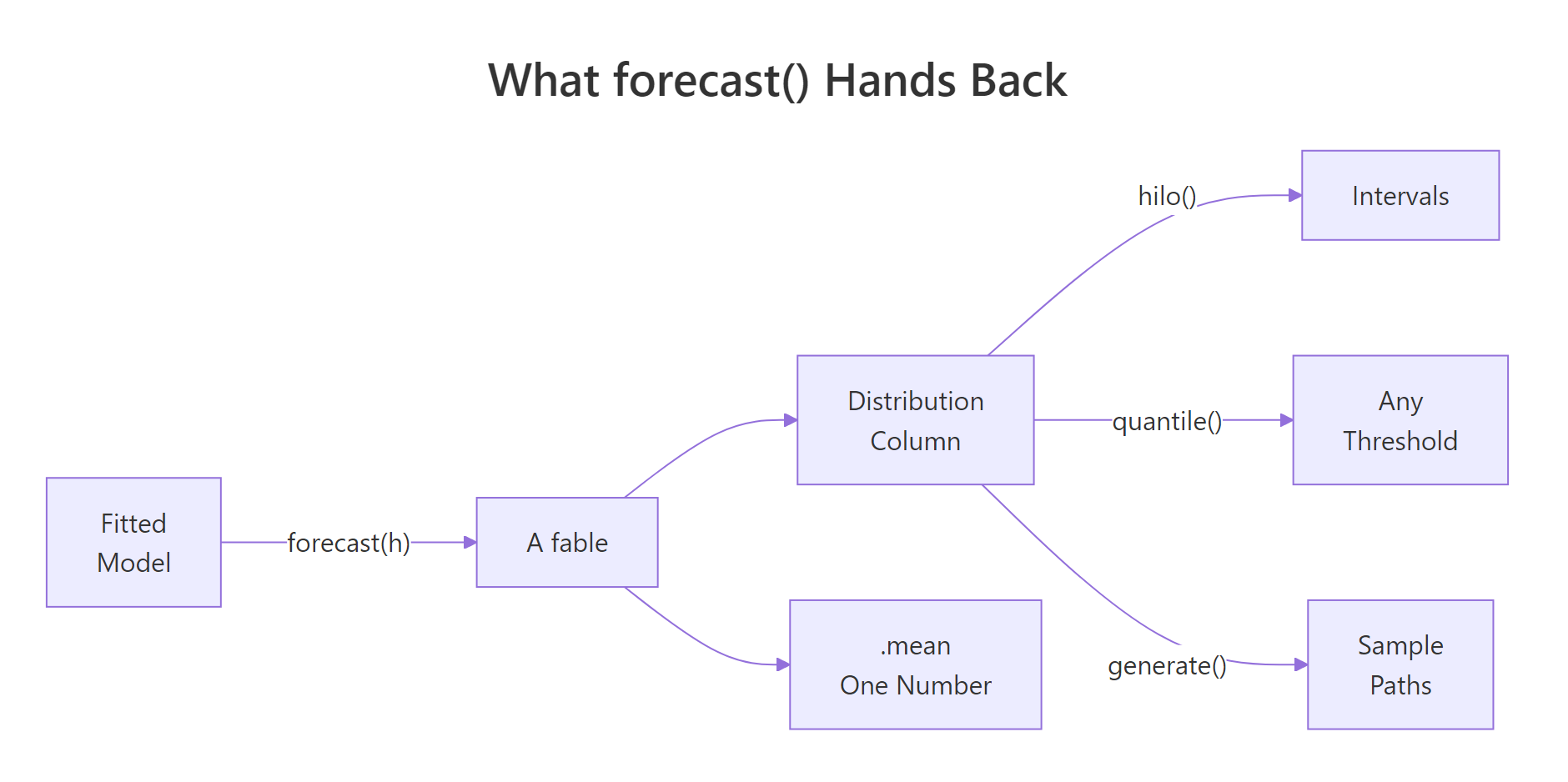
Figure 1: A fable carries the distribution; every other number you want is a question you ask of it.
Try it: Forecast six months ahead with SNAIVE() instead, which just repeats the value from the same month last year. Look at the variance inside each distribution and notice how it behaves compared with the ETS forecast above. The starter fits the model but stops short of forecasting.
Click to reveal solution
Explanation: The centres change month to month because SNAIVE copies last year's value for that month. The variance is stuck at 346 for all six months, because a seasonal naive model one year out has no mechanism for growing uncertainty within the first twelve months. The ETS variances, by contrast, crept upward from 222 to 310 over the same span.
How do you turn a distribution into a prediction interval?
An interval is not a new kind of forecast. It is two quantiles of the distribution you already have. A quantile, also called a percentile when it is written as a percentage, is the value the distribution stays below a stated fraction of the time: the 10th percentile is the value the truth should fall below one time in ten. An 80% interval is the 10th percentile at the bottom and the 90th at the top, leaving 10% of the probability hanging off each end.
The function that does this in fable is hilo(), named for the high and low ends it returns.
hilo(80) added a column of type <hilo>, a small object holding both bounds plus the confidence level they belong to, which is the little 80 printed after the closing bracket. January's forecast is 351, with an 80% interval running from 331.7 to 369.9.
The as_tibble() and select() steps are there purely for display. A fable insists on keeping its key and index columns, so converting to an ordinary tibble first lets you show only the three columns that matter here.
There is nothing mysterious about those bounds. You can rebuild them by hand from the mean and standard deviation we extracted earlier.
Identical to the digit. qnorm(0.9) is the number of standard deviations you step out from the centre of a bell curve to leave 10% in the tail, roughly 1.28. Step that far below the mean and that far above it, and you have captured the middle 80%.
That is the entire formula, and it is worth writing down once.
$$\text{interval} = \hat{y} \pm c \times \sigma$$
Where:
- $\hat{y}$ is the point forecast, the centre of the distribution
- $\sigma$ is the standard deviation of the forecast distribution
- $c$ is a multiplier that depends only on the coverage you asked for
The multiplier is the same for every forecast anyone has ever made with a normal distribution, so it is worth recognising the common values.
| Coverage | Multiplier $c$ |
|---|---|
| 50% | 0.67 |
| 80% | 1.28 |
| 90% | 1.64 |
| 95% | 1.96 |
| 99% | 2.58 |
If you are not interested in the arithmetic, skip ahead. The practical point is simply that hilo() does this for you.
In practice you often want more than one level, and you usually want plain numbers rather than <hilo> objects so you can plot or export them. You cannot call hilo() twice on a fable, because the first call already turned it into an ordinary table. Instead, call hilo() on the distribution column itself, as many times as you like.
unpack_hilo() split each <hilo> object into two ordinary numeric columns and named them after the original column with _lower and _upper appended. Now every bound is a plain number you can do arithmetic on.
Those numeric columns are exactly what a fan chart is made of. Older fable material draws this chart with autoplot(), which recent releases have moved out of the package, so building it by hand is both more portable and more instructive: it shows that the shaded bands are nothing but the interval columns you just created.
The grey line is history through December 2017 and the purple line is the point forecast. The darker band is the 80% interval and the paler one the 95%. The enormous December spike is reproduced by the model, and the band around December is visibly the widest of the year, because a big number carries big absolute uncertainty.
Try it: Produce the 50% interval for fc. Half the time the truth should land inside it, which makes it much narrower than the 80% band.
Click to reveal solution
Explanation: January's 50% interval spans about 20 units against the 80% interval's 38. The multiplier fell from 1.28 to 0.67, so the width fell by roughly half.
How do you ask for any quantile, not just an interval?
An interval answers a two-sided question: where will the truth probably land? Plenty of real decisions are one-sided.
If you are ordering stock for December, you do not care about the lower bound. You care about a single number that is high enough to cover demand almost all of the time. That is a quantile, and quantile() works directly on the distribution column.
One call returned twelve numbers, one per forecast month, because quantile() was applied to the whole column at once. For January, 375.3 is the level that the truth should stay under 95% of the time.
That is more useful inside a table than as a loose vector, so let us put it beside the point forecast.
Read the two columns as two different business answers. If you stock to expected, you run out roughly half the time, because the mean sits in the middle of the distribution. If you stock to cover_95, you run out about one month in twenty. December is the sharpest illustration: the expected value is 727 but covering yourself properly takes 785, an extra 58 million dollars of turnover capacity.
Which column is correct depends entirely on what a mistake costs you. If running out loses a sale forever and holding stock is cheap, you want the high quantile. If stock is expensive and shortages merely annoy people, the mean is closer to right.
If you would rather have these summaries computed up front, forecast() takes a point_forecast argument listing whatever summaries you want as columns.
Each entry in the list becomes a column, named by the list name. Notice that .mean and .median are identical here, which is the signature of a symmetric distribution. Hold onto that, because it is about to stop being true.
Try it: Build a table with the 10th percentile beside the expected value. This is the pessimistic case, the level demand should exceed nine times out of ten.
Click to reveal solution
Explanation: The gap from 332 up to 351 is the same 19 units as the gap from 351 up to the 90th percentile of 370. Perfect symmetry, because this forecast distribution is a plain normal.
What happens when the forecast distribution is not normal?
Everything so far leaned on a normal distribution, which is symmetric by definition. Real series often break that assumption, and retail turnover is a classic case: it cannot go below zero, and it grows by percentages rather than by fixed amounts.
The standard fix is to model the logarithm of the series instead. In fable you write the transformation straight into the model formula, and it handles the reverse trip for you.
The distribution column now reads t(N(5.9, 0.0019)). The t() wrapper means "transformed", and the numbers inside are on the log scale, which is why 5.9 rather than 351. The exponential of 5.9 is about 365, in the right neighbourhood.
Critically, fable did not throw the transformation away. It remembered it, so .mean is still reported in dollars. What you have is a normal distribution living on the log scale, bent into a new shape on the way back to the original scale. Bending a symmetric curve stretches one side more than the other, so the result is no longer symmetric.
You can watch the symmetry break by asking for the mean and the median again.
The mean now sits above the median, every single month, and the gap widens as the forecast horizon grows: 0.38 in September, 0.85 by December. That is the signature of a right-skewed distribution. A few large values far out in the upper tail pull the average up, while the midpoint stays put, because the midpoint only counts how many values sit on each side of it and not how far out they are.
The skew shows up in the intervals too. Here is December's, measured as the distance from the median down to the lower bound and up to the upper bound.
The interval reaches 65.8 units below the median but 72.3 above it. It is lopsided, and correctly so: a series modelled in percentage terms can run further above its typical level than below it, since it can never fall past zero.
For the curious, the two summaries have closed forms. If the log of the value is normal with mean $\mu$ and variance $\sigma^2$, then
$$\text{median} = e^{\mu} \qquad \text{mean} = e^{\mu + \sigma^2/2}$$
The mean carries that extra $\sigma^2/2$ term, which is exactly why it sits above the median and why the gap grows as $\sigma$ grows with the horizon. Skip this if you like; the practical rule is in the warning below.
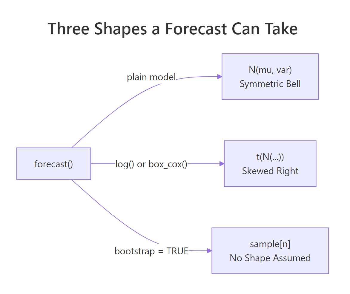
Figure 2: The three distribution shapes fable returns, and what produces each one.
Try it: Confirm the mean beats the median in every one of the twelve months, not just the four shown above. The starter counts how many months qualify; turn that count into a single TRUE or FALSE with all().
Click to reveal solution
Explanation: Because mean() and median() are vectorised over the distribution column, both calls return twelve numbers, and all() collapses the twelve comparisons into one answer. Every month is right-skewed, as the closed form guarantees whenever $\sigma$ is above zero.
What if you do not want to assume a shape at all?
Transforming the series swaps one assumed shape for another. Sometimes you want to assume nothing, and build the spread out of the errors the model has already made.
That is bootstrapping. Those errors are the model's residuals: for each past month, the gap between the value the model fitted and the value that actually turned up. Instead of drawing from a bell curve, you draw randomly from that stored pile of residuals, feed each draw forward as if it were next month's error, and repeat. The only assumption left is that future errors will look like a reshuffling of past ones.
generate() builds these futures one at a time, and they are worth looking at before you collapse them into an interval.
Sixty rows: twelve months times five repetitions. The .rep column labels which future each row belongs to and .sim holds the simulated value. Each one is a complete month-by-month version of 2018 in its own right, not a summary of anything.
Plotting them makes the idea concrete in a way no interval can.
Each coloured line is one plausible 2018. They agree on the shape, a fairly level run through the year and a sharp December peak, and disagree on the month-to-month details. A prediction interval is what you get after running thousands of these and reading off the percentiles at each month.
You do not have to do that by hand. Passing bootstrap = TRUE to forecast() runs the simulations and stores the results as the distribution.
The distribution column now reads sample[1000] instead of N(...). There are no parameters to print, because there is no formula. The distribution literally is a thousand simulated numbers, and hilo() and quantile() answer questions about it by sorting them.
So how much difference does dropping the normal assumption make here? Let us compare the same model both ways.
The two agree closely, which is reassuring rather than disappointing. The bootstrap interval is slightly narrower on both sides, suggesting this model's residuals are a little better behaved than a normal curve would predict. When the two recipes agree, prefer the normal one, because it is computed from a formula in an instant while the bootstrap has to simulate.
The bootstrap earns its keep when they disagree, which happens when residuals are skewed, heavy-tailed, or bunched near a hard floor like zero.
times to 10000 or more before you trust an extreme quantile.Try it: Generate three futures instead of five and confirm the row count matches your expectation.
Click to reveal solution
Explanation: Twelve months times three repetitions is 36 rows. generate() always returns one row per month per repetition, which is why the object grows quickly and why forecast(bootstrap = TRUE) collapses the paths for you rather than handing back five million rows.
How do you tell whether the whole distribution is any good?
RMSE and MAE grade the .mean column and ignore everything else. A model that nails the point forecast while claiming absurd certainty scores exactly the same as one that is honest about its spread, which is no help when you are choosing between them.
The measure that grades the whole distribution is the Continuous Ranked Probability Score, or CRPS. Informally, it rewards putting probability close to what actually happened, and it penalises both being wrong and being overconfident. Lower is better, and it is measured in the same units as the data.
accuracy() computes it when you pass distribution_accuracy_measures.
Note that we scored against dept, the full series, not against train. accuracy() finds the 2018 actuals in there, lines them up with the forecasts by month, and grades each one.
The log model wins with a CRPS of 6.10, the plain ETS is close behind at 6.23, and seasonal naive trails at 7.08. The percentile score tells the same story from a different angle: it grades the forecast at a fixed spread of individual percentiles and averages those grades, where CRPS accounts for the whole curve at once.
It is worth putting the point measures and the distributional one side by side.
Here all three measures agree on the ranking, which is the comfortable case. They do not have to. A model can win on RMSE and lose on CRPS when its point forecasts are sharp but its intervals are far too narrow, and that model will keep surprising you in production even though its headline error looks good.
Try it: Score just the two ETS variants against each other on CRPS, leaving the naive benchmark out.
Click to reveal solution
Explanation: Passing a named list to measures gives you exactly the columns you asked for. The scores match the three-model run because each model is scored independently against the actuals.
Complete Example: turning a distribution into a stock plan
Here is the whole page in one flow, with no new ideas. We fit three candidates, let CRPS pick the winner, use a high quantile of the winner's distribution to set stock cover for every month of 2018, then check what actually happened.
Start by scoring and choosing, without hand-picking the answer.
slice_min() took the row with the lowest CRPS and pull() extracted its name. The transformed model won, which matches what we saw in the previous section.
Now build the plan. The expected column is what we think will happen; the cover column is the level we would actually stock to.
December asks for 785 against an expected 726. That 59 unit buffer is the price of being caught short only one month in twenty.
Finally, the honest part. We held 2018 back at the very start, so we can check the plan against reality instead of trusting it.
Twelve months planned, twelve covered. December came in at 724 against an expected 726, almost exactly on the nose, and comfortably under the 785 cover level.
One caveat worth stating plainly: twelve months is a small sample, so twelve out of twelve is encouraging rather than proof. A 95% level predicts roughly one miss every twenty months, and seeing none across twelve is entirely consistent with a well-calibrated forecast and also with a slightly over-cautious one. Judging calibration properly needs many more forecasts, which is what backtesting is for.
Practice Exercises
Exercise 1: Does the interval widen with the horizon?
Uncertainty should compound the further ahead you look. Raw interval widths hide this for a seasonal series, because December's interval is wide simply because December is big. Compute the 95% interval width for fc as a percentage of the point forecast, alongside the horizon number, and see whether the pattern appears.
Click to reveal solution
Explanation: Once you divide out the seasonal level, the pattern is unmistakable: relative uncertainty climbs steadily from 16.6% one month ahead to 19.0% twelve months ahead. The raw widths were jagged because a 19% band around December's 727 is enormous in absolute terms while a 17% band around February's 284 is small.
Exercise 2: Does an 80% interval really cover 80% of the time?
An 80% interval promises to contain the truth in about eight months out of ten. Test that claim for fc_log against the 2018 actuals. Count how many of the twelve months landed inside the band.
Click to reveal solution
Explanation: All twelve landed inside a band that only promised about ten, which suggests the intervals are wider than they strictly need to be for this year. Do not over-read it: with twelve observations the sampling noise is large, and 2018 was an unremarkable year for this series. The same check across many origins is what turns this from a hint into evidence.
Exercise 3: A question intervals cannot answer
Suppose a supplier contract triggers if total 2018 turnover exceeds 4800 million dollars. Monthly intervals cannot tell you the probability of that, because the total depends on how the months move together. Simulate 2000 futures from fit_log, total each one, and estimate the probability.
Click to reveal solution
Explanation: About 17% of simulated years cleared 4800, so the contract was unlikely but far from impossible. The middle 90% of annual totals ran from 4511 to 4872, and the actual 2018 total came in at 4737, close to the simulated median of 4697. Every number here required whole paths. No collection of twelve monthly intervals could have produced any of them, which is the strongest practical reason to keep generate() in your toolkit.
Frequently Asked Questions
What is the difference between a prediction interval and a confidence interval here?
A confidence interval describes uncertainty about a quantity you are estimating, such as a trend coefficient. A prediction interval describes uncertainty about a single future observation, which includes both the estimation error and the plain randomness of the next data point. Everything hilo() returns is a prediction interval, which is why these bands are much wider than the confidence intervals you may be used to from regression output.
Why does my back-transformed point forecast disagree with .mean?
Because they are different summaries. Exponentiating the log-scale point forecast gives you the median of the forecast distribution, while .mean is the bias-adjusted mean, which sits above it for a right-skewed distribution. Neither is wrong. Use the median when you want the typical month and the mean when the figures will be added into a total, since only means add correctly.
Why does hilo() throw an error the second time I call it?
hilo() on a fable consumes the fable and returns an ordinary tsibble, so the second call has no distribution column left to work with. To get several levels, call hilo() on the distribution column itself inside mutate(), as in mutate(pi80 = hilo(Turnover, 80), pi95 = hilo(Turnover, 95)).
How many bootstrap simulations do I actually need?
For ordinary 80% or 95% intervals, 1000 is normally plenty and the answer barely moves above that. For anything in the far tail, such as a 99.9th percentile or the probability of a rare threshold crossing, push times to 10000 or higher, because an extreme quantile is estimated from only a handful of the simulated draws.
Should I use CRPS instead of RMSE to choose a model?
Use CRPS when the interval matters to the decision, which is most of the time in planning, inventory and risk work. RMSE only grades the point forecast, so it cannot distinguish a model with honest intervals from an overconfident one. Keep reporting RMSE alongside it, since stakeholders recognise it and the two usually agree.
What if my model does not come from fable?
The distribution machinery lives in the distributional package, not in fable, so you can build the same objects yourself. Wrapping your own forecasts and standard errors in dist_normal(), or a matrix of simulated futures in dist_sample(), gives you a column that hilo() and quantile() treat exactly like a fable's own.
Summary
The single idea worth carrying away is that forecast() returns distributions, and every other number is a question you ask of them.
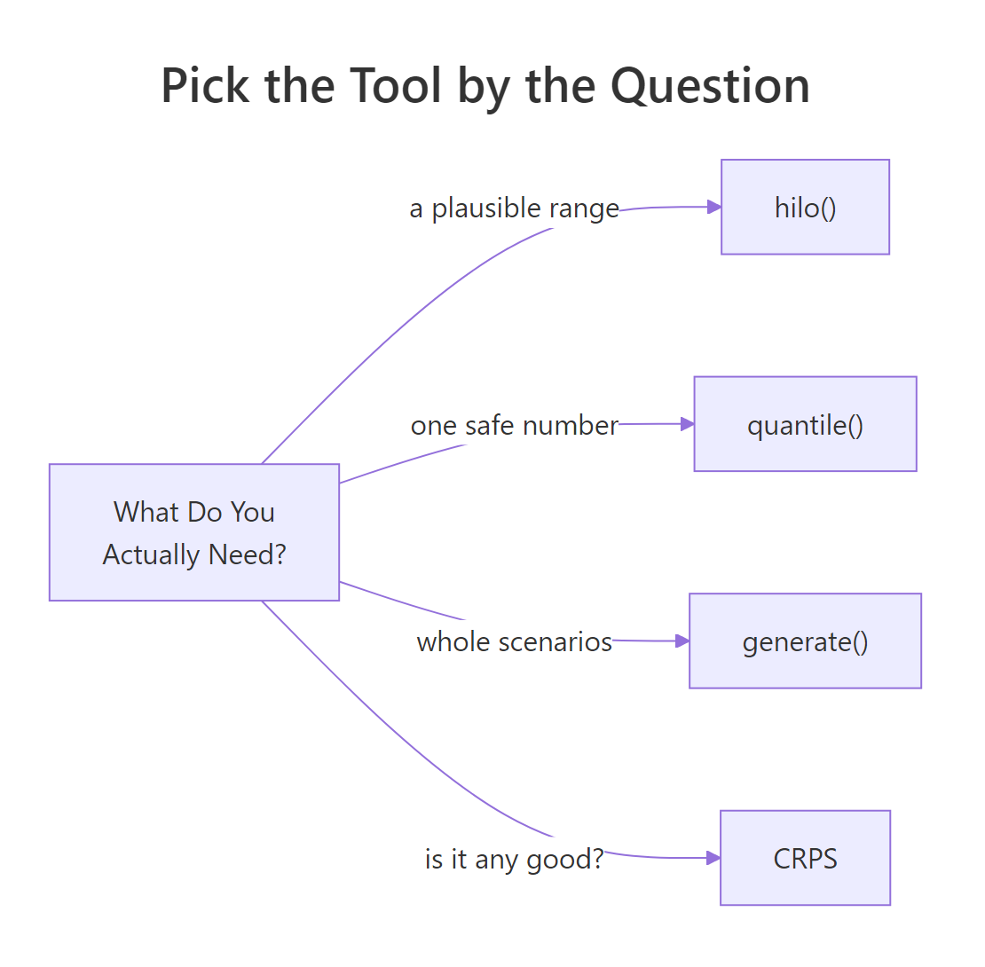
Figure 3: Pick the function by the decision you are making, not by habit.
| Question you are asking | Function | What you get back |
|---|---|---|
| Where will it probably land? | hilo(level) |
A <hilo> interval column |
| I need those bounds as numbers | unpack_hilo() |
Plain _lower and _upper columns |
| What level covers me 95% of the time? | quantile(dist, 0.95) |
One number per forecast period |
| Give me several summaries at once | point_forecast = list(...) |
One column per summary |
| What do individual futures look like? | generate(times =, bootstrap =) |
One row per period per path |
| Drop the normal assumption entirely | forecast(bootstrap = TRUE) |
A sample[n] distribution |
| Is the whole distribution any good? | accuracy(measures = CRPS) |
One score per model |
Five things that will save you time later:
- The numbers inside
N()are the mean and the variance. Take the square root before you reason about spread. .meanis a summary, not the forecast. The forecast is the distribution beside it.- A transformed model gives a skewed distribution, so its mean and median differ, and its intervals are lopsided on purpose.
.meanon a transformed forecast is bias-adjusted, so it is neither the median nor the naive back-transform of the point forecast.- Only sample paths answer path-level questions such as annual totals, peaks, or the chance of crossing a threshold in any month.
References
- Hyndman, R.J. & Athanasopoulos, G. Forecasting: Principles and Practice, 3rd edition, Section 5.5: Distributional forecasts and prediction intervals. Link
- Hyndman, R.J. Non-Gaussian forecasting using fable. Link
- fabletools reference: Compute hilo intervals. Link
- fabletools reference: Produce forecasts, including the
point_forecastandbootstraparguments. Link - fabletools reference: Distribution accuracy measures, including CRPS and the percentile score. Link
- distributional package documentation, the vctrs-based distribution class behind the
<dist>column. Link - Hyndman, R.J. Tidy forecasting in R, the original introduction to the fable framework. Link
- Hyndman, R.J. & Athanasopoulos, G. Forecasting: Principles and Practice, Section 5.9: Evaluating distributional forecast accuracy, the source for the quantile and CRPS definitions. Link
Continue Learning
- fable in R covers the framework this page builds on: tsibbles, mables, and how to fit several models at once.
- Box-Cox and Transformations for Time Series in R goes deeper on choosing a transformation, which is what produced the skewed
t(N(...))distributions above. - Conformal Prediction in R builds forecast intervals from held-out errors instead of a model's own distribution, which is the natural next step when you suspect the model's spread is wrong.