ETS Models in R: Error, Trend, and Seasonal Components
An ETS model builds a forecast from three moving parts: the Error, the Trend, and the Seasonal pattern. That is where the name comes from, E, T, and S. Each part is switched to one of three settings, none, additive, or multiplicative, so a short code like ETS(M,Ad,M) describes the whole model. This one framework covers flat series, trending series, and seasonal business data. This post shows what each letter means, how to fit a model with ets() from the forecast package, how R picks the best one for you, and how to read the forecast it produces.
What does ETS stand for, and why does it matter?
Forecasting a monthly series by hand means juggling three questions at once. Where is the overall level heading? Is there a repeating seasonal shape? And how noisy is the data around that pattern? An ETS model answers all three at the same time, and R fits one in a single line.
ETS stands for Error, Trend, and Seasonal, the three components every ETS model is made of. The letters also nod to the method's origin, because ETS is the modern, statistically grounded form of exponential smoothing. We will use the AirPassengers series: 144 monthly totals of international airline passengers, in thousands, from January 1949 to December 1960. It ships with R, so you already have it. Press Run on the block below.
The very first line is the payoff. ETS(M,Ad,M) is the model R chose on its own, without you telling it anything about the data. Read the three letters in order: M error, Ad trend, M seasonal. In plain English, R decided the noise is multiplicative, the trend is additive but damped (the d), and the seasonal swing is multiplicative. The rest of the printout lists the numbers that define this specific model, and we will unpack every one of them as we go.
For now, notice what just happened. One function call inspected a seasonal series and returned a complete, named forecasting model plus goodness-of-fit scores (AIC, AICc, BIC). That naming is the heart of ETS, and the diagram below shows the anatomy behind the three-letter code.
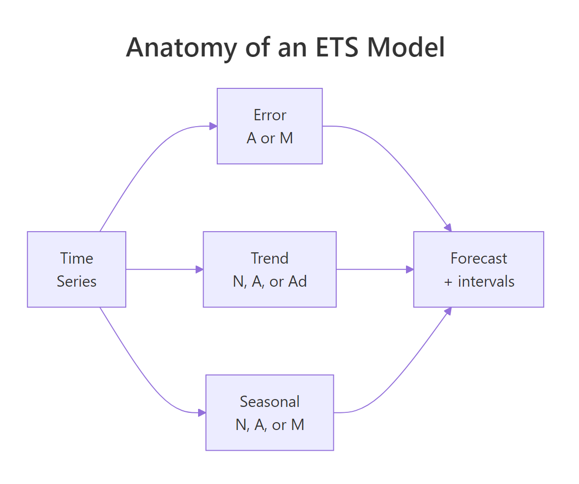
Figure 1: An ETS model splits a series into Error, Trend, and Seasonal parts, then recombines them into a forecast.
Try it: Fit an automatic ETS model to a different built-in series, USAccDeaths (monthly accidental deaths in the US, 1973 to 1978), and print just its three-letter code with $method.
Click to reveal solution
Explanation: For USAccDeaths, R picks ETS(A,N,A): additive error, no trend, additive seasonal. Unlike the airline data, this series has no long-run climb, so the trend slot is set to N.
What do the three letters (E, T, S) actually mean?
Each of the three components can take one of a few settings, and the letter in the code tells you which. Here is the full menu.
- Error (first letter):
Aadditive orMmultiplicative. Additive error means the random wobble is roughly the same size all the way through. Multiplicative error means the wobble grows as the series climbs. - Trend (second letter):
Nnone,Aadditive (a straight-line trend), orAdadditive damped (a trend that flattens out over time). The littledmarks damping. - Seasonal (third letter):
Nnone,Aadditive, orMmultiplicative.
The one idea that trips up beginners is the difference between additive and multiplicative. It is worth slowing down for, because it decides two of the three letters. Additive means the seasonal swing (or the noise) stays a constant size no matter how high the series climbs. Multiplicative means the swing grows in proportion to the level: when the series doubles, the swing roughly doubles too.
You can see which one AirPassengers needs by measuring the size of the seasonal swing early and late in the record. The swing is just the gap between the busiest and quietest month of a year.
The window() function slices out one year at a time. In 1949 the gap between the busiest and quietest month was 44 thousand passengers. By 1960 that same gap had grown to 232 thousand, more than five times larger. The seasonal pattern did not just sit there, it scaled up as air travel grew.
That is the fingerprint of multiplicative seasonality, and it is exactly why ets() set the seasonal letter to M for this series. If the swing had stayed near 44 both years, additive (A) would have been the right call. The diagram below sums up the choice.
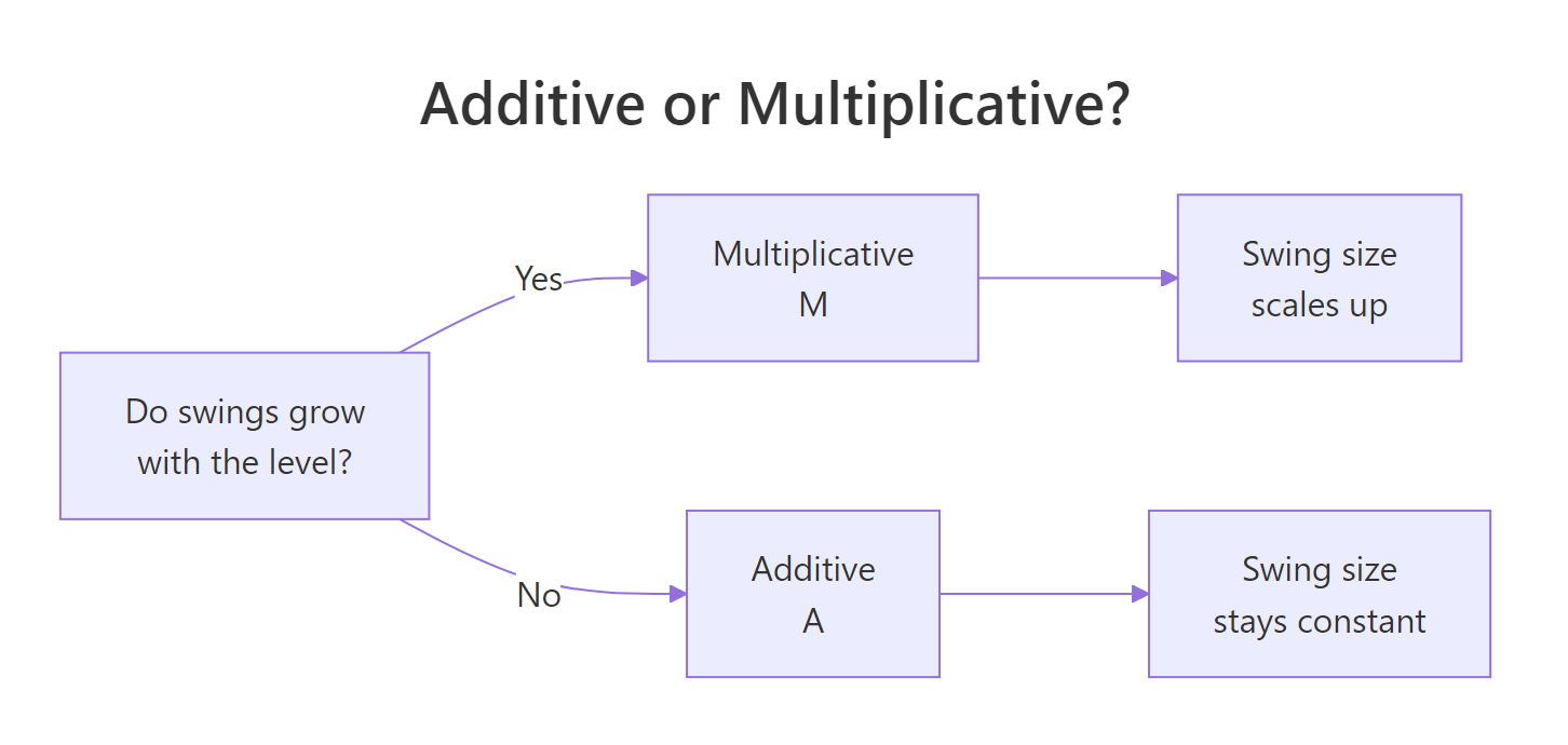
Figure 2: Additive seasonality keeps a constant swing; multiplicative seasonality grows with the level.
Try it: Measure the seasonal swing for USAccDeaths in its first year (1973) and last year (1978). Does the swing grow a lot, or stay roughly steady? Use that to say whether the seasonality looks additive or multiplicative.
Click to reveal solution
Explanation: The swing moves from 3211 to 3592, only a modest change while the additive pattern holds roughly constant. That is why ets() chose A (additive) for the seasonal component of this series, not M.
How many ETS models are there?
Once you know the menu for each letter, counting the models is simple multiplication. The error has 2 settings and the season has 3. The trend has 5: the three you met above (none, additive, additive damped) plus two multiplicative-trend forms (multiplicative and multiplicative damped) that complete the taxonomy but rarely get used. That gives 2 times 5 times 3, which is 30 possible ETS models.
You do not need to memorise all 30. A handful are famous methods you may already have met under other names, and ETS is simply the umbrella that contains them. The table below lists the ones you will actually see.
| ETS code | Error, Trend, Season | Common name |
|---|---|---|
| ETS(A,N,N) | additive, none, none | Simple exponential smoothing (SES) |
| ETS(A,A,N) | additive, additive, none | Holt's linear trend |
| ETS(A,Ad,N) | additive, damped, none | Damped trend method |
| ETS(A,A,A) | additive, additive, additive | Additive Holt-Winters |
| ETS(M,A,M) | multiplicative, additive, multiplicative | Multiplicative Holt-Winters |
| ETS(M,Ad,M) | multiplicative, damped, multiplicative | Damped multiplicative Holt-Winters |
Reading the table top to bottom, the models get richer: no trend and no season at the top, then a trend, then a full seasonal pattern at the bottom. The model ets() chose for the airline data, ETS(M,Ad,M), is the last row, a seasonal method with a gently flattening trend.
You can build any named method by hand by passing its code to the model argument. Here is additive Holt-Winters, ETS(A,A,A), fitted to the airline series.
By passing model = "AAA" you overruled the automatic search and forced an additive model. Notice the seasonal s values are now plain numbers that add to the level (like -29.18 and 66.18), whereas the multiplicative fit in section 1 had seasonal factors near 1 that multiply the level (like 0.89 and 1.23). That is additive versus multiplicative made concrete.
Also compare the two sigma values: 18.05 here versus 0.0392 for the multiplicative fit. They are on different scales (one is in passengers, one is a proportion), so you cannot compare them directly, which is exactly why we need a fair score to choose between models. We build that score in a later section.
Try it: Force multiplicative Holt-Winters, ETS(M,A,M), on the airline series and confirm the code with $method. Pass damped = FALSE so R keeps the plain (undamped) trend you asked for.
Click to reveal solution
Explanation: model = "MAM" requests multiplicative error, additive trend, multiplicative season. Adding damped = FALSE stops R from quietly testing a damped version, so you get the exact ETS(M,A,M) you asked for.
How do you fit an ETS model with ets() in R?
You have already used ets() twice, so here is the whole picture of how it works. Called with just a series, ets(y) searches the candidate models and returns the best one. Called with model = "XYZ", it fits exactly the model you name. There is also a wildcard: the letter Z means "choose this component for me". So ets(y, model = "ZZZ") is the same as the fully automatic call, and ets(y, model = "ZAZ") would fix the trend to additive while auto-selecting the error and season.
To see everything a fitted model holds, wrap it in summary(). It repeats the model description from section 1 and adds a row of accuracy scores at the bottom.
Read the summary in four blocks. First, the model line ETS(M,Ad,M) names the chosen model. Second, the smoothing parameters (alpha, beta, gamma, phi) control how quickly each component reacts to new data, and they get their own section next. Third, the initial states (l, b, s) are the model's best guess at the level, trend, and twelve seasonal factors at the very start of the series in 1949.
Fourth come the scores. sigma is the model's noise size, and AIC, AICc, and BIC measure fit while penalising complexity (lower is better). The final row is the training set error measures, the model's accuracy on the data it learned from. The most readable of these is MAPE, the mean absolute percentage error: 2.86 means the fitted values sit within about 2.9 percent of the actual passenger counts on average, which is a tight fit.
Try it: Pull the level smoothing parameter, alpha, out of the fitted model. The parameters live in fit$par, a named vector, so you can index it by name.
Click to reveal solution
Explanation: fit$par holds every estimated number by name, so fit$par["alpha"] returns the level parameter, 0.7096. The next section explains what that value tells you.
What do the smoothing parameters (alpha, beta, gamma, phi) mean?
Every ETS model keeps a running estimate of the level, the trend, and the seasonal factors, and updates them each time a new observation arrives. The smoothing parameters decide how big each update is. There are four of them, and each one belongs to a specific component.
- alpha controls the level: how fast the baseline adapts to new data.
- beta controls the trend: how fast the slope adapts.
- gamma controls the season: how fast the seasonal shape adapts.
- phi is the damping factor: how quickly the trend flattens toward the horizon.
Every smoothing parameter sits between 0 and 1. A value near 0 means the component barely reacts to the newest point, so it stays smooth and stable. A value near 1 means it chases the latest observation hard, so it is quick to change but jumpier. Let us read the four values from the airline fit.
The story these four numbers tell is clear once you know the scale. alpha is 0.71, fairly high, so the level tracks recent passenger counts closely. beta is 0.02 and gamma is 0.0001, both almost zero, so the trend slope and the seasonal shape are treated as nearly fixed: they were set early and barely drift. phi is 0.98, just under 1, so the trend is damped only gently and keeps most of its slope into the future.
If you want the single equation behind the level update, the simplest ETS model, simple exponential smoothing (SES), makes it concrete. Its forecast is the latest level, and the level is updated like this.
$$\ell_t = \alpha \, y_t + (1 - \alpha)\, \ell_{t-1}$$
Where:
- $\ell_t$ = the updated level after seeing the newest value
- $y_t$ = the newest observed value
- $\ell_{t-1}$ = the previous level
- $\alpha$ = the level smoothing parameter, between 0 and 1
Read it as a weighted average: the new level is a blend of the newest observation and the old level, and alpha sets the mix. At alpha = 0.71, the newest point gets 71 percent of the weight and history gets 29 percent. Trend, season, and damping each add one more update equation of the same shape, which is all a full ETS model really is. If you are not interested in the equation, skip it, because the value of alpha alone already tells you how reactive the level is.
Try it: Extract the seasonal smoothing parameter, gamma, from the fit and round it to 4 places. Given its size, decide whether the seasonal shape is nearly fixed or fast-changing.
Click to reveal solution
Explanation: gamma is 0.0001, so close to zero that the twelve seasonal factors set in 1949 barely change across the whole series. The airline's seasonal shape is stable, even as its overall level climbs.
How does ets() choose the best model automatically?
When you call ets(AirPassengers) with no model, R fits many candidates and needs a fair way to crown a winner. It cannot just pick the model with the smallest errors, because a more complex model can always hug the training data more tightly and then forecast badly. The fix is an information criterion that rewards good fit but charges a penalty for each extra parameter.
R uses the AICc, a small-sample-corrected version of the Akaike Information Criterion. Lower is better. It balances how well the model fits against how many parameters it spends, so it favours a model that explains the data without overfitting. The picture below shows the loop.

Figure 3: How ets() scores every candidate model with AICc and keeps the lowest.
You can reproduce the contest by hand. Fit a few named models, read the aicc value out of each, and sort them. The automatic pick should land at the top.
Sorted smallest first, the winner is auto at 1400.64, the ETS(M,Ad,M) model R selected. The plain multiplicative Holt-Winters (MAM) is a close second at 1403.66, so the gentle damping bought only a small improvement. Additive Holt-Winters (AAA) trails at 1570.73, and simple exponential smoothing (ANN), which ignores trend and season entirely, is far behind at 1733.96. The gap of more than 300 AICc points between ANN and the rest is the numeric proof that this series truly needs its seasonal component.
Try it: Compare the automatic model's AICc against a no-trend, no-season multiplicative model, MNN. The auto model should score much lower.
Click to reveal solution
Explanation: MNN has no trend and no season, so it scores 1674.07, far worse than the auto model's 1400.64. AICc confirms what your eyes already suspect: a flat model cannot describe a climbing, seasonal series.
How do you forecast and read the prediction intervals?
Fitting a model is only half the job. To forecast, pass the fitted model to forecast() and say how many steps ahead you want with h. For monthly data, h = 12 means the next twelve months.
Each row is one month. The Point Forecast is the model's single best guess, so it expects about 442 thousand passengers in January 1961, rising to a summer peak of 613 thousand in July. Notice the forecast is not a smooth line, it carries the seasonal shape forward: summers high, winters low, exactly the pattern the model learned.
The four remaining columns are prediction intervals, the model's honest statement of uncertainty. Lo 80 and Hi 80 bracket the range the model is 80 percent sure the actual value will fall in, and Lo 95 to Hi 95 is the wider, more cautious 95 percent range. For July 1961 the 95 percent interval runs from 513 to 714, so the model is confident July will be busy but cannot pin the exact number.
Two things make these intervals move. They widen the further out you forecast, because uncertainty compounds with distance, and because this is a multiplicative model, they also widen where the level and the seasonal factor are high. That is why the July interval is far wider than the January one. Point forecasts alone hide this, which is why you should always look at the intervals.
Before trusting any forecast, measure how well the model fit the history and whether it left any pattern behind. Two functions do this. accuracy() prints the error scores, and checkresiduals() tests whether the residuals still contain signal.
These are the same training-set error measures the summary printed back in section 4; accuracy() is just the dedicated function for them. Alongside the MAPE of 2.858 (the roughly 2.9 percent average error from before), read the RMSE of 10.75, which puts the typical error in raw units: around 11 thousand passengers. Both are small relative to a series that ranges from 100 to over 600, so the fit is strong.
checkresiduals() runs a Ljung-Box test, whose null hypothesis is that the residuals are pure noise with no leftover pattern. The p-value here is 0.00095, well below 0.05, so we reject that null: some structure remains in the residuals. Running the block also draws the residual diagnostic plots in the panel below the code. In practice ETS(M,Ad,M) is still an excellent, widely used fit for this series, and the failed test is a reminder that even a good model rarely captures a real series perfectly.
Try it: Forecast the next twelve months and read off the single point forecast for the first month, January 1961. The point forecasts live in fc$mean.
Click to reveal solution
Explanation: fc$mean is the vector of point forecasts, so fc$mean[1] is the first, January 1961, at 441.8 thousand passengers. It matches the top row of the forecast table above.
When should you use ETS instead of ARIMA?
ETS is not the only forecasting framework in R. Its main rival is ARIMA, and the two think about a series in different ways. ETS models the level, trend, and season directly. ARIMA models the correlation between a value and its own past values. The table below is a quick guide to which fits your problem.
| Question | ETS | ARIMA |
|---|---|---|
| What it models | Level, trend, and season directly | Correlation with past values |
| Handles seasonality | Yes, additive or multiplicative | Yes, via seasonal terms |
| Needs a stationary series | No | Yes, usually after differencing |
| External predictors | Not supported | Supported (dynamic regression) |
| Always gives a sensible forecast | Yes | Can misbehave if mis-specified |
Reach for ETS when a series has a clear trend and a repeating seasonal shape, which covers most business data like sales, demand, and web traffic. It needs no differencing, and it always returns a stable forecast. Reach for ARIMA when the interesting structure is autocorrelation, or when you need to include external predictors, which plain ETS cannot do.
ETS has real limits worth knowing. It handles only one seasonal period, so it cannot model data with both a weekly and a yearly cycle. It takes no external regressors. And its multiplicative forms need strictly positive data. When you hit those walls, dynamic regression or a model like TBATS takes over.
The forecast package's ets() is the classic interface, but the modern tidyverts stack offers the same model through the fable package's ETS() function. It uses tsibble data and pipes, and it selects the identical ETS(M,Ad,M) with the same parameters. Run this one locally in RStudio, because the fable stack is not available in the in-browser runtime here.
library(fable)
library(tsibble)
library(dplyr)

# Convert the built-in ts into a tsibble, then let ETS() auto-select
air <- as_tsibble(AirPassengers)
fit_fable <- air |>
  model(ets = ETS(value))
fit_fable
#> # A mable: 1 x 1
#>             ets
#>         <model>
#> 1 <ETS(M,Ad,M)>
Calling report(fit_fable) on that fit prints the same smoothing parameters and the same AICc (1400.64) you saw from forecast::ets(), so the two packages agree exactly. Use whichever fits your workflow: forecast for the compact classic interface, fable if you already work in the tidyverse.
Try it: Confirm the Z wildcard. Fit ets() with model = "ZZZ", which asks R to auto-select all three components, and check that its code matches the fully automatic fit from section 1.
Click to reveal solution
Explanation: Z tells R to choose that component itself, so ZZZ is identical to calling ets() with no model at all. Both return ETS(M,Ad,M), confirming the automatic search is exactly the ZZZ case.
Complete Example: forecasting monthly deaths end to end
Let us run the whole workflow once on a fresh series, the way you would in real work: fit on the past, forecast the future you have not seen, and grade the forecast against what actually happened. We will use USAccDeaths and hold out its final year to test on.
The steps are: split the series into a training part (1973 to 1977) and a test part (all of 1978), let ets() pick and fit a model on the training part only, forecast the twelve months of 1978, then compare those forecasts to the real 1978 values with accuracy().
On the training years R chose ETS(M,N,M): multiplicative error, no trend, multiplicative season, a sensible read of a series that cycles hard but has little long-run drift. The accuracy() call now prints two rows because we gave it the held-out test data. The Training set row is the fit on data the model learned from, and the Test set row is the real prize: how the forecast did on the twelve months it never saw.
The test-set MAPE is 2.660, meaning the forecast for unseen 1978 came within about 2.7 percent of the actual monthly deaths. That it barely rose from the training MAPE of 2.459 is the sign of a healthy model: it generalised to new data instead of memorising the past. This split-fit-forecast-grade loop is how you should evaluate any forecast before you rely on it.
Practice Exercises
These combine several ideas from the tutorial. Try each before opening the solution. They use fresh variable names so they will not disturb the fit object from earlier.
Exercise 1: Fit and forecast additive Holt-Winters
Fit an additive Holt-Winters model, ETS(A,A,A), to the full USAccDeaths series, then forecast the next twelve months and print the point forecasts rounded to one decimal. Save the model to my_fit.
Click to reveal solution
Explanation: Forcing model = "AAA" gives additive Holt-Winters. The forecast carries the additive seasonal shape into 1979, peaking in July at 10734 and dipping in February at 7541, mirroring the yearly cycle in the data.
Exercise 2: Prove multiplicative beats additive here
For the airline series, fit both multiplicative Holt-Winters (MAM) and additive Holt-Winters (AAA) with damped = FALSE, read the AICc from each, and print them together. Which error type does AICc prefer for this series?
Click to reveal solution
Explanation: Multiplicative Holt-Winters scores 1403.66 against additive's 1570.73, a gap of 167 AICc points in favour of multiplicative. This is the numeric version of the growing-swing pattern you measured in section 2: because the airline's seasonal swing scales with its level, a multiplicative model fits far better.
Exercise 3: Let a train and test split pick the model
Split the airline series into a training set through 1958 and a test set from 1959 on. Fit an automatic ETS model and a forced additive model (AAA) on the training set, forecast the test period from each, and compare their test-set RMSE. Which generalises better?
Click to reveal solution
Explanation: On the held-out 1959 to 1960 data, the automatic model (again ETS(M,Ad,M)) has a test RMSE of 72.55 versus 91.22 for the forced additive model. The multiplicative, damped model does not just fit the past better, it forecasts the unseen future more accurately too.
Frequently Asked Questions
What is the difference between ETS and Holt-Winters?
Holt-Winters is not a separate framework, it is one family inside ETS: the models that carry a seasonal component. Additive Holt-Winters is ETS(A,A,A) and multiplicative Holt-Winters is ETS(M,A,M). ETS is the wider umbrella that also covers simple exponential smoothing, Holt's linear trend, and the damped-trend variants, all under a single naming scheme.
Do I need to make my series stationary or difference it first?
No. Unlike ARIMA, ETS models the level, trend, and season directly, so it needs no differencing and no stationarity check. Pass the raw ts object straight to ets() and it fits.
Why did ets() choose a multiplicative model for my data?
It chooses multiplicative when the seasonal swing (or the noise) grows as the series climbs, the way the airline swing grew from 44 in 1949 to 232 in 1960. If your swing stays roughly constant as the level rises, ets() picks an additive model instead. AICc makes the final call by scoring the candidate models against each other.
Can ETS handle more than one seasonal cycle?
No. ets() models a single seasonal period, so it cannot capture both a daily and a weekly cycle in hourly data at once. For multiple seasonalities reach for TBATS, or for dynamic regression with ARIMA errors when you also need external predictors.
What does the little "d" in ETS(M,Ad,M) mean?
The d marks a damped trend. A plain additive trend (A) keeps its full slope into every future step, while a damped additive trend (Ad) flattens that slope the further out you forecast, controlled by the phi parameter. Damping keeps long-horizon forecasts from climbing to unrealistic values.
Summary
ETS gives you one clean framework for forecasting: pick a setting for the Error, the Trend, and the Seasonal component, and a short code names the whole model. The ets() function does the picking for you and returns a model you can read, forecast, and check. The workflow below is the loop to remember.

Figure 4: The end-to-end ETS forecasting workflow, from plot to residual check.
| Idea | What to remember |
|---|---|
| The name | ETS is Error, Trend, Seasonal, the state-space form of exponential smoothing |
| The code | Three letters, like ETS(M,Ad,M): error, trend, season, each set to N, A, or M (Ad means damped) |
| Additive vs multiplicative | Additive keeps a constant swing, multiplicative grows the swing with the level |
| The taxonomy | 2 x 5 x 3 = 30 models in theory; ets() searches a stable subset of about 15 to 18 |
| Fitting | ets(y) auto-selects; ets(y, model = "AAA") forces a model; Z means auto |
| Parameters | alpha, beta, gamma, phi are learning rates from 0 (stable) to 1 (reactive) |
| Selection | ets() minimises AICc, which rewards fit and penalises complexity |
| Forecasting | forecast(fit, h) gives point forecasts plus 80 and 95 percent prediction intervals |
| Checking | accuracy() scores the fit; checkresiduals() tests for leftover pattern |
| Limits | One seasonal period, no external predictors, positive data for multiplicative models |
With those pieces you can fit an ETS model, explain exactly what it assumes about your series, and produce a forecast with honest uncertainty bands, all in a handful of lines.
References
- Hyndman, R.J., & Athanasopoulos, G. (2021). Forecasting: Principles and Practice, 3rd edition, Chapter 8: Exponential smoothing. OTexts. Link - the canonical free textbook treatment, with the full state-space equations behind ETS.
- Hyndman, R.J., & Athanasopoulos, G. Innovations state space models for exponential smoothing (FPP3 section 8.5). Link - spells out the innovations state-space form and the ETS(Error,Trend,Season) taxonomy this post summarises.
- forecast package reference: the
ets()function. Link - the argument-by-argument reference for everyets()option, includingmodelanddamped. - Hyndman, R.J., Koehler, A.B., Snyder, R.D., & Grose, S. (2002). A state space framework for automatic forecasting using exponential smoothing methods. International Journal of Forecasting, 18(3), 439-454. Link - the original paper defining the framework that ets() automates.
- Hyndman, R.J., & Khandakar, Y. (2008). Automatic time series forecasting: the forecast package for R. Journal of Statistical Software, 27(3). Link - explains the automatic AICc model-selection algorithm ets() runs under the hood.
- fable package: the
ETS()function reference. Link - the tidyverts equivalent shown in the last section, for tidyverse workflows.
Continue Learning
- Exponential Smoothing in R: the smoothing ideas that ETS formalises, from simple to Holt's method, with the update equations spelled out.
- Holt-Winters in R: a deeper look at the seasonal methods that ETS(A,A,A) and ETS(M,A,M) generalise.
- Time Series Forecasting in R: where ETS fits among the other forecasting tools, including ARIMA and how to compare them fairly.