ETS vs ARIMA in R: Which Forecasting Model Should You Use?
ETS and ARIMA are the two workhorse forecasting model families in R, and both run in a single line with the forecast package. ETS builds a forecast from a series' structure (its level, trend, and seasonality), while ARIMA builds one from the correlations between a value and its own recent past. This guide shows how each works, why you must never compare them with AICc, and how a fair accuracy test picks the winner.
What is the core difference between ETS and ARIMA?
Give R a monthly time series and two single lines produce two finished forecasters. But which one should you trust? Before you can compare them, you need to see what each model is actually doing. Let's fit both to the same classic dataset, read off the models they choose, and then unpack why those two choices are so different.
We'll use AirPassengers, a dataset built into R: monthly totals of international airline passengers from 1949 to 1960. It has a clear upward trend and a strong yearly season (summer peaks, winter dips), so it is a perfect stress test for any forecaster. Both functions we use here, ets() and auto.arima(), live in the forecast package and pick their own model automatically.
Two lines, two very different answers. ets() returned a label made of letters, ETS(M,Ad,M). auto.arima() returned a set of integer orders that read as ARIMA(2,1,1)(0,1,0)[12]. We will decode both labels in the next two sections. For now, the point is that they describe the same data in completely different languages.
Here is the intuition behind that difference. ETS looks at the series and asks "what is the current level, is it trending, and what is the seasonal pattern?" It then extrapolates that structure forward. ARIMA asks a different question: "after I remove the trend and season by differencing, how does each value relate to the values just before it?" It then models those leftover correlations. One works from the visible shape of the series; the other works from the correlations between each value and the ones just before it.
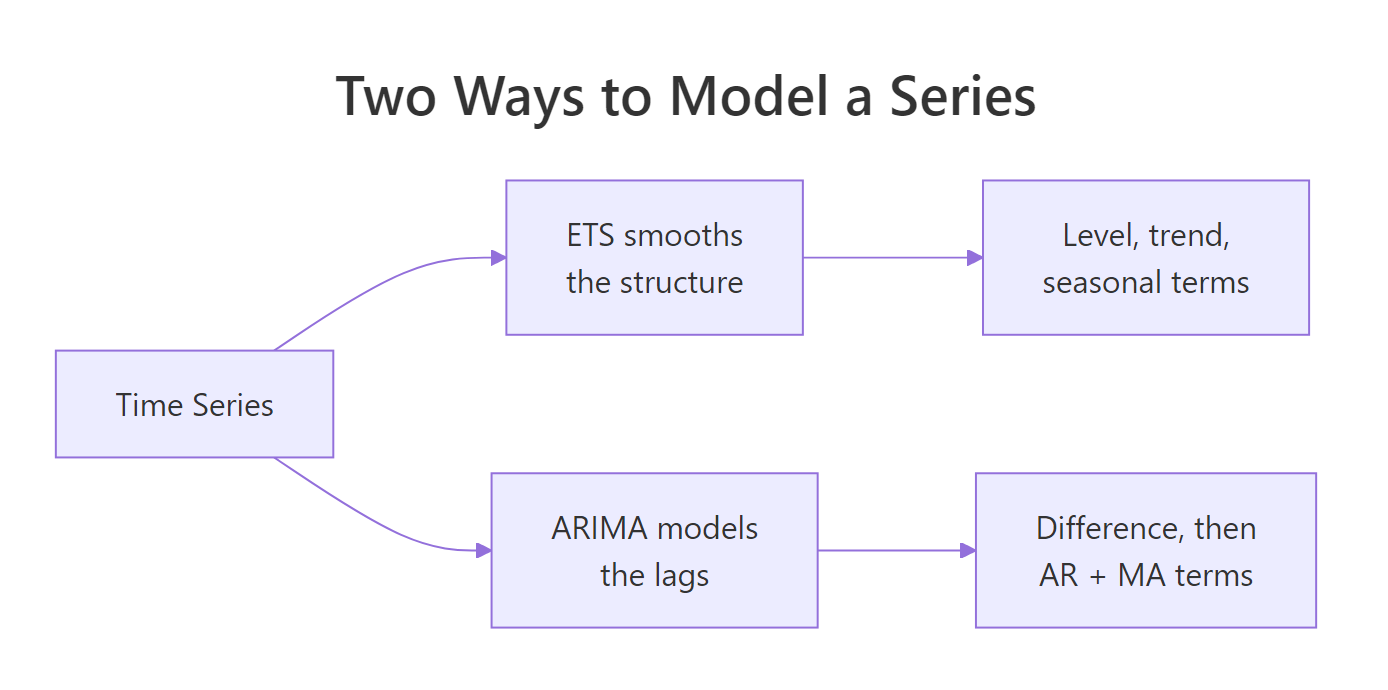
Figure 1: ETS and ARIMA start from the same series but model it in opposite ways.
Try it: Fit both models to USAccDeaths (monthly accidental deaths in the US, also built into R) and print the two model labels. Do the two functions agree on how seasonal the series is?
Click to reveal solution
Explanation: ETS chose ETS(A,N,A): additive error, no trend, additive season. ARIMA chose ARIMA(0,1,1)(0,1,1)[12]. Both detected the yearly season (the A in ETS, the seasonal (0,1,1)[12] in ARIMA), but they encoded it in their own ways.
How does ETS model a time series?
ETS stands for Error, Trend, Seasonal, the three ingredients it uses to build a forecast. The label ETS(M,Ad,M) is just those three ingredients described one at a time: the error is Multiplicative, the trend is Additive and damped, and the season is Multiplicative. Each slot can be A (additive), M (multiplicative), or N (none), which is how one function covers dozens of model shapes.
What does "multiplicative" mean here? It means the seasonal swings and the error grow in proportion to the level of the series. Look at AirPassengers and you can see it: the summer peaks in 1960 are much taller than the peaks in 1949, because the whole series is bigger. A multiplicative season captures that "swings scale with size" behaviour, which additive models cannot.
The engine underneath ETS is exponential smoothing. Its simplest form updates a running estimate of the level after every new observation:
$$\ell_t = \alpha \, y_t + (1 - \alpha)\, \ell_{t-1}$$
Where:
- $\ell_t$ = the smoothed level at time $t$ (the model's current sense of "where the series is")
- $y_t$ = the actual value observed at time $t$
- $\ell_{t-1}$ = the previous level estimate
- $\alpha$ = the smoothing weight, between 0 and 1
The single idea to take away: $\alpha$ decides how much the newest observation matters. A high $\alpha$ trusts recent data and reacts fast; a low $\alpha$ leans on the past and stays smooth. Trend and season have their own smoothing weights, $\beta$ and $\gamma$. If the equation is not your thing, skip it, the printed parameters below tell the same story.
Let's print the fitted model to see those weights R estimated.
Read the smoothing parameters top to bottom. alpha = 0.7096 is fairly high, so the level tracks recent months closely. beta = 0.0204 is tiny, meaning the trend changes very slowly and steadily. gamma = 1e-04 is almost zero, which says the seasonal shape is stable year to year and barely needs updating. The Initial states block holds the starting level l, starting trend b, and the twelve seasonal factors s (one per month). At the bottom sit the information criteria, including AICc, which we return to shortly.
There is a fourth parameter, phi = 0.98. That is the damping factor, the d in Ad.
phi parameter (here 0.98) gently pulls the trend toward flat as the forecast horizon grows, so ETS does not extrapolate a straight line forever. This usually produces more realistic long-term forecasts than an undamped trend.Try it: Fit ets() to austres (quarterly Australian resident numbers) and read off its three-letter label. Which trend and season types did it pick?
Click to reveal solution
Explanation: ETS(M,Ad,A) means a multiplicative error, an additive damped trend, and an additive season. The Ad again signals a damped trend, and this time the season is additive rather than multiplicative.
How does ARIMA model a time series?
ARIMA describes a series through its own past values instead of through visible structure. Its label has three numbers for the non-seasonal part and three more for the seasonal part: ARIMA(p,d,q)(P,D,Q)[m]. Here is what each letter counts, using our fitted ARIMA(2,1,1)(0,1,0)[12]:
- p (here 2): autoregressive terms, how many recent values feed into the prediction.
- d (here 1): how many times the series is differenced to remove trend.
- q (here 1): moving-average terms, how many recent forecast errors feed in.
- P, D, Q (here 0, 1, 0): the same three ideas applied to the seasonal pattern.
- m (here 12): the season length, twelve months for monthly data.
The middle letter, the "I" for Integrated, is the key to ARIMA. Differencing means replacing each value with the change from the value before it. Do that once and a rising trend flattens out. d = 1 here means one round of ordinary differencing, and D = 1 means one round of seasonal differencing (each month minus the same month last year). ARIMA needs the series to be stationary first: no trend, no season, and a roughly constant mean and spread over time. Differencing is how it gets there.
Let's print the full fitted ARIMA to see its estimated coefficients.
The Coefficients block lists the estimated weights: two autoregressive terms (ar1, ar2) and one moving-average term (ma1), each with a standard error underneath. sigma^2 is the estimated variance of the model's one-step errors, and the bottom row shows the information criteria. Notice there is no alpha or gamma here; ARIMA speaks entirely in AR and MA coefficients, not in smoothing weights. That is the same series as before, described in a totally different vocabulary.
d and D orders are ARIMA's built-in way of handling trend and season. If you manually difference or remove the trend before calling auto.arima(), you can double-difference the series and get worse forecasts. Feed it the raw series.Try it: How much differencing does AirPassengers actually need? Use ndiffs() for ordinary differencing and nsdiffs() for seasonal differencing to check.
Click to reveal solution
Explanation: Both return 1, which matches the d = 1 and D = 1 that auto.arima() chose. These helper functions run statistical tests to decide how much differencing makes the series stationary, and auto.arima() calls them internally.
Why can't you compare ETS and ARIMA with AICc?
Here is the trap that catches almost everyone. Both models print an AICc value, and lower AICc means a better model, so it feels obvious to fit both, compare the two AICc scores, and keep the smaller one. That reasoning is wrong, and it will steer you to the worse forecaster.
Let's look at the two numbers side by side.
By this logic ARIMA (1018) crushes ETS (1401), so you would throw ETS away without a second thought. Do not. These two numbers are not measured on the same ruler.
AICc is built from each model's likelihood (a measure of how well the model fits the data it was trained on), and the two families compute that likelihood in different ways. Our ETS model uses multiplicative errors, so its likelihood is defined on the relative scale of the data. The ARIMA model works on the differenced series, so its likelihood is defined on that transformed scale. Comparing the two AICc values is like comparing a temperature in Celsius to one in Fahrenheit by their raw numbers. AICc is genuinely useful, but only for ranking models inside one family: ETS against other ETS models, or ARIMA against other ARIMA models.
Try it: Put both AICc values into a single named vector so they are easy to read together, rounded to one decimal place. (This is only to display them, not to pick a winner.)
Click to reveal solution
Explanation: The vector displays both scores clearly, but remember the whole point: their difference tells you nothing about which model forecasts better. For that we need the next section.
How do you fairly compare ETS and ARIMA in R?
If AICc cannot referee this match, what can? The answer is the same test you would trust for any forecaster: hide the most recent part of the series, forecast it, and measure the error against the values the model never saw. This is a train and test split, and it is the fair comparison every serious forecaster uses.
We'll train both models on AirPassengers up to the end of 1958, then ask each to forecast the final two years, 1959 and 1960, which they were never shown. The window() function slices a time series by date.
Now the comparison is honest, because both models are judged on the exact same unseen data. Here is what each column means in plain terms:
- RMSE (root mean squared error): typical error size in passengers, punishing big misses harder. Lower is better.
- MAE (mean absolute error): average error size in passengers. Lower is better.
- MAPE (mean absolute percentage error): average error as a percentage of the actual value. Lower is better.
- MASE (mean absolute scaled error): error scaled against a naive seasonal forecast, so it carries no units. Lower is better.
On every single metric, ETS wins: lower RMSE (72.55 versus 74.25), lower MAE, lower MAPE, and lower MASE. Remember that ARIMA had the far better AICc? On the data that actually matters, the held-out future, ETS is the better forecaster here. That is exactly why AICc could not be trusted to choose between them.
A picture makes the difference concrete. Let's plot both forecasts against the real 1959-1960 values.
The chart (which draws when you run the block) shows both coloured forecast lines tracking the black actual series, with ETS staying a little closer through the seasonal peaks. Seeing the forecasts overlaid is often more convincing than any single error number.
tsCV() function in the forecast package repeats this holdout across many cut points and averages the errors, giving a sturdier verdict. It is slower because it refits the model many times, so start with a single split and graduate to tsCV() when the decision is important.Try it: Add a baseline. Seasonal naive (snaive()) just repeats last year's value for each month. Score it on the same test set and compare its MASE to the two models above. Did ETS and ARIMA earn their complexity?
Click to reveal solution
Explanation: Seasonal naive scores RMSE 76.99 and MASE 2.49, worse than both ETS (2.21) and ARIMA (2.40). So both real models beat the "just repeat last year" baseline on this holdout, with ETS the strongest of the three.
When should you use ETS vs ARIMA?
You now have the honest workflow: fit both, and let a holdout decide. But you often want a starting instinct before running the test. This table sums up where each family tends to shine.
| Consideration | ETS | ARIMA |
|---|---|---|
| What it models | Level, trend, season directly | Autocorrelation after differencing |
| Stationarity needed | No | Yes (differencing handles it) |
| Multiplicative seasonality | Handles it natively | Needs a log or Box-Cox transform first |
| Extra predictors (regressors) | Not supported | Supported via the xreg argument |
| Auto-selection function | ets() |
auto.arima() |
| Reads most naturally when | The series has clear trend and season | The series is driven by its own recent history |
A widespread myth says ARIMA is the more general, more powerful family, so it must be the safer default. It is not true. As the diagram below and the numbers above both show, the right choice depends on the series, not on a ranking.
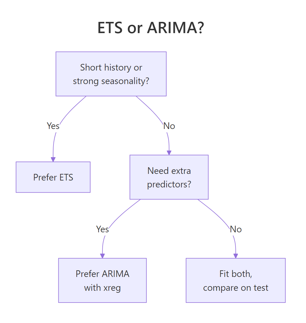
Figure 2: A quick heuristic for which model to reach for first.
The two families genuinely overlap, though. Some simple ETS models are exactly equal to specific ARIMA models, which is why they often forecast alike. These equivalences come from the forecasting textbook by Hyndman and Athanasopoulos:
| ETS model | Equivalent ARIMA model |
|---|---|
| ETS(A,N,N) | ARIMA(0,1,1) |
| ETS(A,A,N) | ARIMA(0,2,2) |
| ETS(A,Ad,N) | ARIMA(1,1,2) |
But the overlap is only partial. Multiplicative ETS models, like the ETS(M,Ad,M) we fit, have no ARIMA equivalent at all. And many stationary ARIMA models have no ETS equivalent, because every ETS model is non-stationary by design. Neither family contains the other, which is the real reason you should try both.
One practical move often beats picking a single winner: average the two forecasts. Let's average the ETS and ARIMA predictions on our AirPassengers holdout and score the blend.
The blended RMSE is 72.70, sitting between ETS (72.55) and ARIMA (74.25). On this particular series the average did not beat ETS alone, which is an honest and useful lesson: averaging often helps, but it is not a guaranteed free win. You still have to measure it on held-out data, exactly as with any single model.
ets() and auto.arima(), forecast a holdout, and compare RMSE or MASE. It costs two extra lines and removes all the guesswork about which family "should" win.Try it: Turn the decision into two lines of code. Use the models already fit above (ets_fc and arima_fc) and print each one's test MASE next to its name so the winner is obvious at a glance.
Click to reveal solution
Explanation: ETS has the lower MASE (2.21 versus 2.40), so it is the winner on this holdout. Wrapping it in a named vector makes the comparison readable in one line.
Practice Exercises
These pull together everything above: you fit both families, hold out the most recent data, then score them on real out-of-sample error. Use fresh variable names so you do not overwrite the tutorial objects.
Exercise 1: Judge both models on a new series
Repeat the fair comparison on USAccDeaths. Train both ets() and auto.arima() on all data up to the end of 1977, forecast the twelve months of 1978, and print each model's test-set RMSE. Which family wins on this series?
Click to reveal solution
Explanation: Here ARIMA edges out ETS (RMSE 288.83 versus 289.62), the opposite of the AirPassengers result. That is the whole point of testing: the winner changes with the data, so you must check, never assume.
Exercise 2: Write a reusable model picker
Write a function pick_model(y, h) that takes any time series y and a horizon h, holds out the last h observations, fits both families on the rest, and returns a small data frame of each model's test MASE. Run it on AirPassengers with h = 24.
Click to reveal solution
Explanation: The function bundles the whole fair-comparison recipe into one reusable call. Point it at any series and horizon and it returns the head-to-head MASE, so you never have to eyeball two model printouts again.
Exercise 3: Test whether averaging beats both
Using USAccDeaths from Exercise 1, average the ETS and ARIMA forecasts and compare the blend's test RMSE against each single model. Does the average win here?
Click to reveal solution
Explanation: This time the average wins outright: RMSE 283.84, lower than both ETS (289.62) and ARIMA (288.83). Blending two decent-but-different forecasts often cancels their opposing errors, which is why forecast averaging is a favourite trick in practice. As always, the holdout proves it rather than assumes it.
Frequently Asked Questions
Should I always use ETS instead of ARIMA because it won here? No. ETS was the better forecaster on AirPassengers, but ARIMA won on USAccDeaths in Exercise 1. There is no family that is better in general, so the honest habit is to fit both and let a holdout decide for the series in front of you.
Can I use ETS or ARIMA if my series has no seasonality? Yes, both handle non-seasonal data. On a series with no repeating yearly pattern, ets() returns N in its seasonal slot (for example ETS(A,A,N)), and auto.arima() simply leaves the seasonal orders at zero. You call the two functions exactly the same way you did above.
My data has an extra predictor like price or temperature. Which model takes it? ARIMA does, through the xreg argument of auto.arima(), which lets you add outside variables alongside the series' own past. Plain ets() has no equivalent, so when an outside predictor matters to your forecast, ARIMA is the family that can use it.
How much history does ARIMA need before it will difference the season? Seasonal differencing (D = 1) needs at least two full seasonal cycles to estimate, so roughly two years of monthly data or two years of quarterly data at a minimum. On a shorter series auto.arima() will usually leave D at zero because there is not enough repetition to measure a stable season.
Why did auto.arima() pick a model that lost my test-set comparison? auto.arima() chooses the model with the lowest in-sample AICc, which rewards fit on the training data, not accuracy on future data it has never seen. Those two goals often agree, but not always, which is exactly why you still run a train and test holdout before trusting a model.
Summary
ETS and ARIMA are two different languages for describing the same time series, and the only fair way to choose between them is an out-of-sample accuracy test.
| Dimension | ETS | ARIMA |
|---|---|---|
| Core idea | Smooth the level, trend, and season | Model autocorrelation after differencing |
| R function | ets() |
auto.arima() |
| Needs stationarity | No | Yes (via the d and D differencing orders) |
| Extra predictors | No | Yes (xreg) |
| Compare models with AICc | Within ETS only | Within ARIMA only |
| Compare ETS vs ARIMA | Never with AICc; use a train and test holdout | Same: use held-out RMSE, MAE, or MASE |
Key takeaways:
- Fit both, it is cheap.
ets()andauto.arima()each take one line and choose their own model. - Never compare their AICc. The two likelihoods live on different scales, so a lower AICc across families means nothing.
- Judge on held-out data. Split the series, forecast the tail, and compare RMSE or MASE on the part neither model saw.
- The winner is data-dependent. ETS won on
AirPassengers; ARIMA won onUSAccDeaths. Test every time. - Consider averaging. Blending the two forecasts sometimes beats either alone, but confirm it on a holdout.
References
- Hyndman, R.J. & Athanasopoulos, G. - Forecasting: Principles and Practice, 3rd ed. Section 9.10: ARIMA vs ETS. Link
- Hyndman, R.J. & Athanasopoulos, G. - Forecasting: Principles and Practice, 3rd ed. Chapter 8: Exponential smoothing. Link
- Hyndman, R.J. & Athanasopoulos, G. - Forecasting: Principles and Practice, 3rd ed. Chapter 9: ARIMA models. Link
- Hyndman, R.J. et al. - Forecasting with Exponential Smoothing: The State Space Approach. Springer (2008). Link
- Hyndman, R.J. - forecast package reference (
ets,auto.arima,accuracy,tsCV). CRAN. Link - R Core Team - R datasets documentation (
AirPassengers,USAccDeaths). Link
Continue Learning
- ETS Models in R: Error, Trend, and Seasonal Components - the full ETS letter system and how
ets()chooses each component. - Exponential Smoothing in R: ses() and the Alpha Parameter - the smoothing engine underneath ETS, one parameter at a time.
- Choosing a Forecasting Model in R - the broader workflow for picking among all the common forecasting methods.