Changepoint Detection in R: the changepoint Package and PELT

A changepoint is the moment a time series stops behaving one way and starts behaving another. Changepoint detection is the job of finding those moments automatically, and in R the standard tool is the changepoint package, whose PELT algorithm searches every possible way of cutting a series into segments and returns the best one exactly, at close to linear cost.

Most tutorials on this topic hand you cpt.mean(), print a list of numbers, and stop. You are left with an algorithm you cannot argue with and a penalty setting you cannot justify. This guide goes the other way. You will write the search by hand in about six lines of base R, watch it land on an answer, and only then meet the package that does the same thing properly. After that the package output stops being a black box.

Everything below uses either a dataset that ships with R itself or a series you simulate in one line from a fixed seed. The numbers you see are the numbers you will get.

What is a changepoint, and why does the exact date matter?

In 1898 the British began building a dam at Aswan. R ships with Nile, the annual flow of the river measured at Aswan from 1871 to 1970, and somewhere inside that record the river's typical flow drops and never comes back. You could squint at a plot and guess the year. Three lines of R will find it for you, and tell you how big the drop was.

Read that block line by line. The second line rescales the series so that it is measured in units of its own standard deviation. That step matters more than it looks: cpt.mean() uses a cost function that assumes the year-to-year noise has a variance of 1, and the Nile is measured in the hundreds, so without the rescaling the algorithm reads ordinary wobble as evidence of change. Only the division by sd() does that work; subtracting the mean first just centres the numbers on zero and never changes which split wins. The section on spread changes below shows exactly what goes wrong when you skip the division. The third line runs the search. cpts() then returns the index of the last observation before the change, which is 28, and time(Nile)[28] converts that index into the year 1898. The final line reports the average flow on each side of the split.

So the algorithm says the Nile's average annual flow fell from about 1098 units to about 850, a drop of roughly 23 percent, starting in 1899. It found the dam without being told that a dam existed.

Now look at the same result as a picture, because the eye is what convinces people in a report.

The two horizontal bars are the segment means, and the dashed vertical line is the changepoint. Notice that the year-to-year wobble is large: the standard deviation of the whole series is 169 units. The drop of 248 units is only about one and a half of those wobbles, which is precisely why eyeballing this is unreliable and why you want an algorithm that weighs the evidence.

How does an algorithm decide where the change happened?

You do not have to take the package on trust, because the idea underneath it fits in a few lines of base R. Start with a way of scoring a single stretch of data. A natural score is how badly that stretch is described by one flat line at its own average, which is the sum of squared deviations from the mean. Small score means the stretch really is flat and uniform.

The first number is the cost of insisting that the whole Nile record is one flat series. The second is the cost of allowing two flat stretches that meet at 1898. Cutting the series in that one place removes 1,237,700 units of cost, which is nearly 44 percent of the total. That is the arithmetic behind "something happened in 1898".

Of course we picked 1898 because we already knew the answer. The honest version tries every possible cut and keeps the best.

That is the entire idea. We built a vector holding the cost of every one of the 97 possible two-segment splits, asked which.min() which entry is smallest, and got index 28. No package was involved, and the answer is identical to the one cpt.mean() gave in the opening block.

It helps to see the whole cost curve rather than only its minimum, because the shape tells you how confident the answer is.

The curve has one deep, clean valley around 1898. A series with no real changepoint gives a shallow, wandering curve with no obvious floor, and a series with several changes gives several local dips. Plotting this curve is a cheap sanity check that costs you one line.

Now for the problem that makes this whole field interesting. If cutting once is good, why not cut twice? Or ninety-nine times?

Give every observation its own segment and the cost falls to exactly zero, because a single number always sits perfectly on its own average. Cost alone will therefore always prefer more changepoints, right up to the absurd extreme of one per observation. Any usable method has to charge a fee for each cut.

Figure 1: How a changepoint search scores one candidate segmentation.

That fee is called the penalty, and it turns the search into a single optimisation. Among all possible numbers of changepoints and all possible positions for them, find the combination with the lowest total of segment costs plus fees.

$$\min_{m,\ \tau}\ \left\{\ \sum_{i=1}^{m+1} \mathcal{C}\!\left(y_{(\tau_{i-1}+1):\tau_i}\right) \ +\ \beta m\ \right\}$$

Where:

• $m$ is the number of changepoints, which the algorithm chooses rather than you
• $\tau_1 < \tau_2 < \dots < \tau_m$ are the positions of those changepoints
• $\mathcal{C}(\cdot)$ is the cost of one segment, the seg_cost() we wrote above
• $\beta$ is the penalty charged for each changepoint kept

If you are not interested in the notation, the sentence before it is all you need: score every segmentation by how badly it fits plus how many cuts it used, and keep the winner.

How do you read what cpt.mean() gives you back?

The package returns an S4 object rather than a plain vector, and each accessor answers a different question. The clearest way to meet them is on the simplest possible search: AMOC, short for At Most One Change, which does exactly the brute-force sweep you just wrote by hand.

Four accessors, four answers. cpts() gives the changepoint positions as indices. param.est() returns the fitted parameter for each segment, here the two means, which are in standardized units because we fed the function standardized data. nseg() counts segments, always one more than the number of changepoints. seg.len() gives the length of each segment, so 28 years before the change and 72 after.

For a human-readable version of all of it at once, print the object's summary.

Every line here is a decision that was made on your behalf, and each one is an argument you can override. The type of change was the mean. The search method was AMOC. The cost function assumed normally distributed data. The penalty was MBIC with a value of 13.81551. Segments were allowed to be as short as one observation, and at most one changepoint was permitted.

That penalty number is worth pinning down, because "MBIC" is otherwise just a label.

The headline penalty value is exactly $3\log n$, which for 100 observations is 13.81551. The logLik() call then shows the fit two ways: 225.4143 is twice the negative log-likelihood of the fitted two-segment model, and 233.0231 is that same figure after a penalty charge has been added. Subtract them and the gap is 7.6088, which is log(28) + log(72), the last line of the block. (The final digit differs only because each printed figure was already rounded.)

The two accessors are therefore reporting different pieces of the same charge. pen.value() gives the flat $3\log n$ term, and the penalised column of logLik() adds the segment-length term on top of the raw fit.

That is not a coincidence, and it is the whole point of MBIC. A plain BIC charges a flat fee per changepoint no matter where you put it. MBIC additionally charges for lopsided splits, because a changepoint that carves off a tiny sliver at the very edge of a series is usually noise rather than a real regime change. The segment-length term is how it expresses that scepticism.

What makes PELT better than binary segmentation?

AMOC finds one changepoint. Real series often have several, and the moment you allow more than one the search space explodes: with 400 observations there are astronomically many ways to place an unknown number of cuts. Two strategies dominate, and the difference between them is the difference between "definitely the best answer" and "usually the best answer".

Binary segmentation is the greedy strategy. Find the single best split, then split each resulting half the same way, and keep going until no split pays for itself. It is fast and intuitive. PELT is the exact strategy: it evaluates the optimal segmentation of the whole series without ever committing to a split it might later regret.

Start with a well-behaved example where both work. Here is a series with four regimes and three genuine changepoints, at 100, 200 and 300.

PELT nailed all three positions exactly and recovered means of -0.10, 3.12, -0.90 and 1.92 against true values of 0, 3, -1 and 2. Note that no scaling was needed here, because the simulated noise already has a standard deviation of 1.

Binary segmentation gets the same answer on this data, provided you let it look for enough changepoints.

The Q argument caps how many changepoints binary segmentation is allowed to find. Set it to 5 and the method finds the three that exist. Set it to 2 and it returns only the first two splits it made, along with a warning advising you to raise Q. PELT has no equivalent argument, because it decides the number for itself.

Now the case that actually separates them. Consider a series that sits at zero, spikes up for fifteen observations, returns to roughly zero, dips down for fifteen observations, and settles back at zero. The true changepoints are at 40, 55, 95 and 110.

PELT recovered all four changepoints perfectly. Binary segmentation, allowed up to eight, found only the last two and missed the entire first half of the story.

The third line explains why. Binary segmentation's opening move is exactly the AMOC search, and AMOC's single best split for this series is at index 95. Having cut there, binary segmentation now looks at observations 1 to 95, a stretch containing an upward spike near the start whose effect on the segment average is diluted by forty quiet observations on each side. That diluted signal no longer clears the penalty, so the search stops. The first split was locally optimal and globally destructive, and the greedy method has no mechanism for taking it back.

Both spikes are real and roughly equal in size, 2.95 up and 3.40 down. Only one of them survives the greedy search.

So why did anyone ever use the greedy method? Because exhaustively checking every segmentation used to be unaffordable.

For a series of 20,000 observations there are 200 million candidate segments to price. The naive exact method pays roughly that cost, growing with the square of the series length, which is why it was abandoned in practice.

PELT's contribution is a pruning rule that keeps exactness while removing almost all of that work. In plain terms: as the algorithm sweeps forward it maintains the best segmentation found so far for every position. If some old candidate position is already more expensive than the current best, even before you charge it the penalty it would still owe for the extra changepoint, then that candidate can never win at any later point in the series. It is deleted permanently and never priced again. When changepoints occur at a roughly steady rate, so much gets pruned that the total work grows about linearly with the length of the series.

How do you choose the penalty?

The penalty is the one number that changes your answer most, so it deserves more thought than accepting a default. Compare the standard options on the four-regime series, where we know the truth is three changepoints.

One series of 400 observations containing three real changes, and the answers range from 3 to 399. No penalty at all gives the degenerate answer we predicted earlier: 399 changepoints, one between every pair of observations. AIC charges too little and returns 16, keeping thirteen spurious splits. BIC, Hannan-Quinn and MBIC all recover exactly 3.

The pattern generalises. AIC is designed for prediction and tolerates extra parameters, so it over-segments. BIC and its relatives charge a fee that grows with the length of the series, which makes them consistent: as you collect more data they stop inventing changepoints. MBIC adds the lopsidedness charge you saw earlier, making it the most sceptical of the three.

Rather than trusting any label, watch what happens as you turn the penalty dial by hand.

This is the single most informative diagnostic in changepoint analysis. At a penalty of 1 the method finds 135 changes, at 2 it finds 57, at 5 it finds 8, and from 10 all the way to 200 it finds exactly 3 and refuses to budge. A twentyfold change in the penalty does not move the answer.

That flat stretch is what a real signal looks like. Spurious changepoints are cheap to buy and disappear as soon as the price rises, whereas genuine ones survive an enormous range of prices. If your answer changes every time you nudge the penalty, you do not have a changepoint, you have a preference.

Doing that sweep by refitting on a grid is wasteful, and the package offers a purpose-built alternative called CROPS, which computes every distinct segmentation across a whole penalty range in one pass.

CROPS reports that between penalties of 5 and 200 there are only three distinct answers. Penalties from 5 to about 6.11 give 8 changepoints, a narrow band up to 6.27 gives 6, and everything from 6.27 to 200 gives 3. The cpts.full() matrix lists those answers as rows, padded with NA, and the third row is the familiar 100, 200, 300.

Notice how the extra changepoints in the first row (23 and 30) and the second row (314, 318) are clustered and short-lived. They exist only in a penalty band of width 1.27, while the true answer holds across a band of width 194.

The package also draws this for you as an elbow plot.

The plot shows the number of changepoints against the penalty. You are looking for the elbow, the point after which paying more penalty stops buying you a meaningfully simpler model. Here the curve flattens hard at 3 and stays there.

What if the spread changes instead of the level?

So far every example has been about the average level moving. Plenty of real changes are not about the level at all. A machine starts vibrating more without running hotter on average. A market becomes turbulent while drifting nowhere. For those you need a different cost function, and the package gives you one function per question.

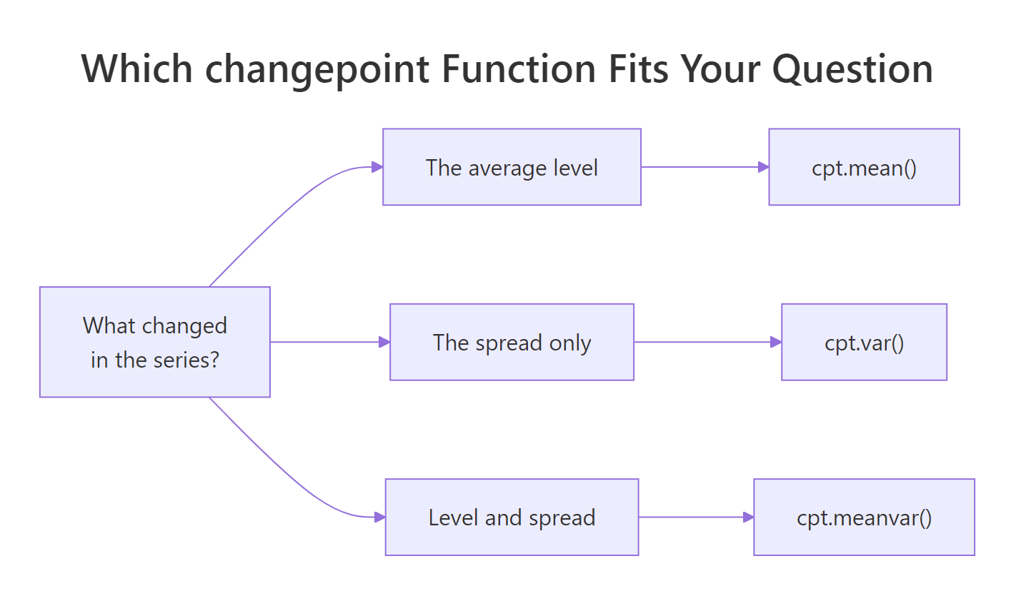
Figure 2: Match the question you are asking to the cpt function that answers it.

Here is a series whose average never moves but whose standard deviation triples halfway through.

cpt.var() found the break at index 195, five observations from the truth at 200, and estimated segment variances of 0.86 and 8.54. Taking square roots gives standard deviations of 0.93 and 2.92 against true values of 1 and 3. Variance is estimated less precisely than a mean, so being five observations out on 400 is a good result rather than a poor one.

Now watch what the mean-change function does with the same data, which is the failure mode worth burning into memory.

Two lines, and neither one reports the change that actually happened. Scaled properly, cpt.mean() returns integer(0), no changepoints, and that answer is correct as far as it goes: the mean genuinely never changes. It answered the question it was asked, which was about the level. It simply has no way to tell you that the spread tripled.

Unscaled, it reports 31 changepoints, and every one is an artefact. The default cost assumes the noise has variance 1, so the second half of the series, where the variance is really 9, does not fit that assumption at all. The search responds the only way it can: it cuts the second half into many short segments, each with its own fitted mean, because a staircase of shifting levels is the closest a mean-change model can get to describing extra spread.

When both the level and the spread can move, cpt.meanvar() estimates them jointly.

Both changepoints were found exactly. The three segments have means of 0.00, 4.00 and 4.17 and variances of 1.02, 0.22 and 4.23, against true means 0, 4, 4 and true variances 1, 0.25 and 4. The second changepoint at 300 is a pure change in spread: the mean is 4 on both sides of it, so cpt.mean() has nothing to find there. cpt.var() would find that one, but it looks only for changes in spread, so it would say nothing about the level shift at 150, and that unmodelled shift would inflate the variance it estimates for the stretch containing it. Asking about both at once is what recovers the full story.

Which assumptions quietly break changepoint detection?

Everything so far has fed the algorithm independent observations that are flat within each segment. Real time series routinely violate that, and the failures are dangerous because they look like results. Here is a series with no changepoints whatsoever: it is pure AR(1) noise, where each value is 0.9 times the previous value plus a fresh random shock.

Seven changepoints, every one of them fictional. Nothing about the process that generated the data ever changed. The problem is that the cost function assumes observations are independent, so a long run of above-average values is treated as strong evidence of a raised mean. In an autocorrelated series, long runs happen all the time simply because each value inherits most of the previous one.

The last line diagnoses the problem in advance. acf() reports lag 0 first, and that entry is always 1 because every observation matches itself, so the number to read is the second one: the correlation between each observation and the one immediately before it is 0.911. A value that high means the series drifts in long runs rather than bouncing around independently, which is precisely the pattern the cost function misreads as a shift in level. Checking it costs one line, and you can do it before you fit anything.

A trend causes the same failure through a different route.

This series has no changepoints either. It slopes gently upward the whole way. PELT is forced to describe a ramp using flat segments, so it does the only thing it can and approximates the slope with a two-step staircase. The changepoints at 106 and 210 are just where the steps look best, and they would move if you extended the series.

The obvious first reflex is to forbid short segments, which helps but does not cure.

Requiring at least 50 observations per segment cuts the seven fake AR changepoints down to two. Two fake changepoints is better than seven and still wrong. minseglen is a useful guard against slivers, not a treatment for dependence.

The real fixes match the violation:

1. Autocorrelation. Model it away first, then look for changes in what remains. Fit an ARIMA model and run the changepoint search on its residuals, or difference the series if the dependence comes from a random walk.
2. Trend. Difference the series, or regress out the trend and search the residuals. A changepoint in the slope is a different question that needs a segmented-regression tool rather than cpt.mean().
3. Non-normal or heavy-tailed data. The default cost assumes normality. The companion changepoint.np package provides cpt.np(), which uses a nonparametric cost that makes no distributional assumption, at the price of some sensitivity.
4. Short segments. Set minseglen to the shortest regime you would consider real. If a change lasting five observations is not actionable for you, do not let the algorithm report one.

The Nile passes the check comfortably enough to trust, with lag-1 autocorrelation of 0.498. Some of even that is caused by the changepoint itself, since 28 above-average years followed by 72 below-average years is autocorrelated by construction.

How do the pieces fit into one workflow?

Put the whole thing together on the Nile, in the order a careful analysis actually runs. First, check the assumption before choosing a method.

The first line is the 0.498 from the previous section, moderate rather than the 0.911 that broke the AR example, so nothing here disqualifies cpt.mean(). The second line adds something new: differencing flips the autocorrelation to -0.402, the signature of over-differencing a series that was not a random walk. That tells us the Nile is better described as a level that shifted than as a series that wanders, which is exactly the situation cpt.mean() is built for.

Second, confirm the answer is not an artefact of the penalty.

Across the entire penalty range from 3 to 60, a twentyfold span, CROPS finds exactly one distinct segmentation containing exactly one changepoint. This is as strong as penalty evidence gets. Compare it to the four-regime simulation, where the same call produced three competing answers.

Third, report the result as a table a non-specialist can read, rather than a vector of indices.

The helper converts changepoint indices into segment boundaries, then computes summary statistics per segment. It takes the fitted object, the original unscaled series, and optionally a vector of labels such as years, which is why the table reads in calendar years rather than positions.

The output is the finished analysis. The Nile ran at an average of 1098 units with a standard deviation of 135 from 1871 to 1898, then at 850 with a standard deviation of 125 from 1899 to 1970. The within-segment variability barely changed, which supports the choice of cpt.mean() over cpt.meanvar(): what happened at Aswan moved the level, not the volatility.

Practice Exercises

Exercise 1: Date the New Haven warming

nhtemp holds the mean annual temperature in Fahrenheit at New Haven, Connecticut, from 1912 to 1971. Standardize it, fit PELT, and report the year of the changepoint along with the average temperature before and after it.

Exercise 2: Automate the penalty plateau

Write a function smallest_penalty(series, max_cpts) that searches a grid of manual penalty values and returns the smallest penalty producing no more than max_cpts changepoints, along with the count it actually produced. Test it on sim with max_cpts = 3.

Exercise 3: Segment a market into volatility regimes

EuStockMarkets holds daily closing prices for four European indices. Convert the DAX column into daily log returns in percent, then use cpt.var() with minseglen = 100 to split the period into volatility regimes. Report a table with the start and end time of each regime and its daily standard deviation.

Frequently Asked Questions

When should I use cpt.mean() rather than cpt.meanvar()? Use cpt.mean() when you are confident the variability stays constant and only the level can shift, since it estimates fewer parameters and is therefore more sensitive to genuine level shifts. Use cpt.meanvar() when either could move or when you are not sure. The cost of guessing wrong is silent, as the variance example above showed.

Why does cpt.mean() return dozens of changepoints on my data? Almost always because your series is not on a unit-variance scale. The default Normal cost assumes the noise has variance 1, so a series measured in thousands looks impossibly erratic and gets cut into many short segments. On the raw Nile, cpt.mean(Nile, method = "PELT") returns 94 changepoints; dividing by the standard deviation first returns 1. Either standardize, or switch to cpt.meanvar(), which estimates the variance rather than assuming it.

Should I ever prefer binary segmentation to PELT? Rarely. PELT is exact and comparable in speed on typical series, so the guarantee is close to free. Binary segmentation is still useful when you want to force an exact number of changepoints via Q, or on extremely long series where the pruning happens to be ineffective because changepoints are very sparse.

Can the changepoint package detect changes in real time? Not directly. The cpt.* functions are offline methods: they see the whole series at once and can revise where an earlier changepoint sits after seeing later data. For streaming detection you want sequential methods, though re-running PELT on a growing window is a workable approximation when new data arrives in batches.

How much data do I need per segment? For a mean shift, roughly 20 to 30 observations on each side gives reliable detection when the shift is about one standard deviation, and less if the shift is larger. Variance changes need more, typically 50 or more, which is why the DAX example used minseglen = 100. Set minseglen to the shortest regime that would actually be meaningful to you. Bear in mind too that the index you get back is an estimate of the location, not an exact date: the variance example above landed on 195 when the truth was 200, and short segments or small shifts make that error larger. Report the changepoint as approximately when the change happened, not precisely.

What if my data are not normally distributed? The default cost assumes normality, and heavy tails make it report changepoints where a few extreme values sit. Use the companion changepoint.np package and its cpt.np() function, which uses a nonparametric cost based on the empirical distribution and makes no distributional assumption. You trade a little sensitivity for robustness.

How is this different from a structural break test? They answer overlapping questions from different directions. Structural break tests, such as those in the strucchange package, are usually framed around a regression model and ask whether its coefficients are stable over time. Changepoint methods are framed around the distribution of the series itself. If your question is "did the relationship between x and y change", reach for a structural break test; if it is "did this series change", reach for the changepoint package.

Summary

Figure 3: The order of operations that keeps changepoint results trustworthy.

The five things worth remembering:

1. A changepoint search is cost plus a fee. Score each segment by how badly one flat line fits it, then charge a fee per cut and minimise the total. Without the fee, the answer is always a cut everywhere.
2. PELT gives the exact answer. Its pruning rule discards only candidates that provably cannot win, so it matches an exhaustive search while running close to linear in the length of the series.
3. cpt.mean() assumes unit variance. This one detail causes more wrong results than everything else combined. Standardize, or use cpt.meanvar().
4. Report the plateau, not the default. Sweep the penalty or run CROPS. An answer that survives a twentyfold range of penalties is a finding; one that changes with every nudge is not.
5. Check the acf first. Autocorrelation and trend both manufacture confident, entirely fictional changepoints. One line of diagnosis prevents a whole class of published mistakes.

References

1. Killick, R., Fearnhead, P. and Eckley, I.A. Optimal Detection of Changepoints with a Linear Computational Cost. Journal of the American Statistical Association 107(500), 2012. The original PELT paper. Link
2. Killick, R. and Eckley, I.A. changepoint: An R Package for Changepoint Analysis. Journal of Statistical Software 58(3), 2014. Link
3. changepoint package reference manual, CRAN. Full argument documentation for every cpt.* function. Link
4. cpt.mean documentation, R Project. Argument-by-argument reference for mean changepoints. Link
5. cpt.meanvar documentation, R Project. Covers the Normal, Gamma, Exponential and Poisson test statistics. Link
6. Haynes, K., Eckley, I.A. and Fearnhead, P. Computationally Efficient Changepoint Detection for a Range of Penalties. The CROPS algorithm. Link
7. changepoint.np package, CRAN. Nonparametric changepoint detection for non-normal data. Link
8. cpt.np documentation, R Project. The nonparametric cost function in practice. Link

Continue Learning

• Anomaly Detection in Time Series in R covers the other half of this problem, finding individual observations that do not belong rather than moments when the rules changed.
• Time Series Decomposition in R shows how to strip out trend and seasonality, which is exactly the preprocessing that stops those two artefacts from manufacturing fake changepoints here.
• ARIMA in R is the tool for modelling the autocorrelation that broke the AR example above, so you can run a changepoint search on residuals that actually satisfy the independence assumption.