GARCH Models in R: Volatility Forecasting with rugarch
A GARCH model forecasts how volatile a series will be tomorrow by blending three things: a baseline level of variance, how big yesterday's surprise was, and how volatile yesterday already was. In R you fit one with the rugarch package, and this guide builds the model from scratch first so that none of it stays a black box.
Almost every tutorial on this topic hands you ugarchfit(), prints a wall of numbers, and moves on. You end up with output you cannot interpret. Here we do it the other way round. You will simulate a GARCH process by hand, write its likelihood function yourself, estimate it with optim(), and only then meet the package that does all of it for you. By that point you will be able to read the package output line by line and say what each number is.
Everything uses EuStockMarkets, a dataset that ships with R itself. No downloads, no API keys, and the numbers you see below are the numbers you will get.
Why do stock returns break ordinary time series models?
Regression and ARIMA models rest on a quiet assumption: the typical size of the error stays the same throughout the sample. Financial returns violate that assumption more obviously than almost any other data you will meet. Run the block below and look at the shape of the noise, not its direction.
That block turned prices into returns and drew them. The diff(log(...)) step converts a price series into log returns, which is the standard way to measure a percentage change, and multiplying by 100 puts everything in percentage points. So a value of -0.933 means the index fell about 0.93% that day.
Now look at the picture. The series is not a uniform band of noise. There are long stretches where the line barely moves, and then bursts where it swings far in both directions for weeks at a time. Big moves arrive next to other big moves. Calm days arrive next to other calm days. That bunching is called volatility clustering, and it is the single fact this whole article exists to model.
Let us put a number on it by comparing an early calm stretch to a later turbulent one.
Both windows come from the same index and both are 250-ish trading days long. Yet a typical day in the second window swings 1.6 times as far as a typical day in the first. A model that assumes one fixed standard deviation for the whole sample has to split the difference, and will be wrong in both periods: too high during the calm stretch, too low during the turbulent one.
Here is the part that surprises most people. The direction of returns really is close to unpredictable, exactly as the efficient-market story claims. It is the size that is predictable. We can show both at once by comparing the autocorrelation of returns with the autocorrelation of squared returns.
An autocorrelation measures how much today's value tells you about the value some days later, on a scale from -1 to 1, where 0 means "nothing at all". Read down the two columns. The returns column hovers around zero: yesterday's return tells you essentially nothing about today's. The squared_returns column is positive at every single lag and reaches 0.17. Squaring throws away the sign and keeps only the magnitude, so that column is asking "does a big move yesterday predict a big move today?" The answer is a clear yes.
Try it: Check whether the same calm-versus-turbulent pattern shows up in the UK's FTSE index. Build FTSE log returns the same way, then compute the ratio of the standard deviations over the same two windows.
Click to reveal solution
Explanation: The FTSE shows the same effect as the DAX but milder, a ratio of 1.25 against the DAX's 1.6. Volatility clustering is a property of markets in general, though its strength varies from index to index.
What exactly is a GARCH model?
The name is an acronym worth unpacking, because each letter is a real design decision:
- Conditional Heteroskedasticity means the variance changes over time, and that we are modelling it conditional on what we already saw. "Heteroskedasticity" is just the technical word for "non-constant variance".
- Autoregressive means today's variance depends on its own past values.
- Generalized means we let it depend on past variances, not only on past shocks.
A GARCH model has two separate equations, and keeping them separate is the key to not getting lost. The mean equation describes the return itself, and it is usually almost trivial:
$$r_t = \mu + \varepsilon_t, \qquad \varepsilon_t = \sigma_t z_t, \qquad z_t \sim D(0, 1)$$
The variance equation is where all the action is. This is GARCH(1,1), the workhorse:
$$\sigma_t^2 = \omega + \alpha_1 \varepsilon_{t-1}^2 + \beta_1 \sigma_{t-1}^2$$
Where:
- $r_t$ = the return on day $t$
- $\mu$ = the average return, typically tiny for daily data
- $\varepsilon_t$ = the surprise, or shock, on day $t$, meaning how far the return landed from its average
- $\sigma_t$ = the volatility on day $t$, which is what we forecast
- $z_t$ = a standardised random draw with mean 0 and variance 1
- $D$ = the distribution those draws come from, which you choose when you fit the model. A normal distribution is the default; we will see later why a fatter-tailed one usually fits returns better
- $\omega$ (omega) = a constant baseline level of variance
- $\alpha_1$ (alpha) = how strongly yesterday's shock feeds into today's variance
- $\beta_1$ (beta) = how much of yesterday's variance carries over
The (1,1) counts how many past terms of each kind we use: one past shock, one past variance. In plain words, the variance equation says: today's variance is a baseline, plus a bit of yesterday's surprise, plus most of yesterday's variance.
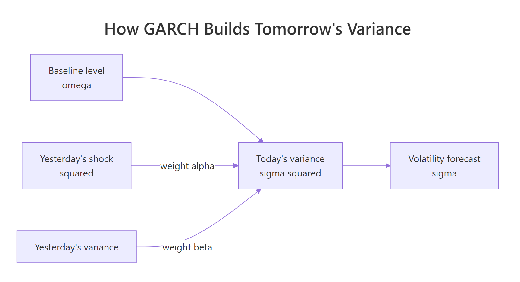
Figure 1: Tomorrow's variance is a weighted blend of three things: a baseline, yesterday's shock, and yesterday's variance.
The parameters are not free to be anything. All three must be non-negative, otherwise the model could predict a negative variance, which is meaningless. And $\alpha_1 + \beta_1$ must stay below 1, for a reason we will see shortly.
The clearest way to understand a recursion is to run it. Below we generate a GARCH(1,1) series ourselves, one day at a time, with parameters we choose.
The loop is the model. On each pass it computes today's variance from yesterday's shock and yesterday's variance, then draws today's shock by scaling a standard random number by today's volatility. Follow rows 2 to 4 in the output: the shocks are small, so sigma2 drifts steadily downward. Then row 5 delivers a shock of 1.01, and sigma2 turns around and climbs at row 6. That is volatility clustering, produced by the recursion rather than assumed.
Let us open up a single step to see the three contributions separately.
The three pieces add to the total, and notice how lopsided the split is. The carried-over variance contributes 0.918 while yesterday's fresh news contributes only 0.218. With beta at 0.85, volatility mostly remembers. New information nudges the level; it rarely resets it. That is why volatility drifts in long waves instead of jumping around at random.
Now the reason $\alpha_1 + \beta_1 < 1$ matters. That sum is called persistence, and it controls whether the process settles down to a stable long-run variance:
$$\text{Unconditional variance} = \frac{\omega}{1 - \alpha_1 - \beta_1}$$
With persistence at 0.95 the formula predicts a long-run variance of exactly 1.0, and our 1,500 simulated days delivered 0.82. The gap is ordinary sampling variation: a highly persistent process wanders slowly, so 1,500 days is not a lot of independent information about its average level. Push the simulation to 100,000 days and the two numbers converge.
Try it: Two GARCH processes can share the same persistence but behave completely differently. Simulate one that reacts hard to news (alpha 0.25, beta 0.70) and one that mostly remembers (alpha 0.05, beta 0.90), then compare how much each one's volatility path bounces around, measured by the standard deviation of sigma itself.
Click to reveal solution
Explanation: Both have persistence 0.95 and the same long-run variance, yet the volatility path of the first is three times as jumpy. Alpha controls how violently the model reacts to news; beta controls how long it remembers. Persistence alone does not tell you the character of the process.
How do you test whether your returns actually need a GARCH model?
Fitting GARCH to data with no volatility clustering wastes parameters and can mislead you. So test first. There are two tests worth running, and the crucial thing is that they answer different questions.
The Ljung-Box test asks whether a series has any leftover autocorrelation. Run it on returns and it asks about predictable direction. Run it on squared returns and it asks about predictable size.
A p-value is the probability of seeing a pattern this strong if there were really no pattern at all. Small p-value means the pattern is real. The first test returns 0.78, so there is no evidence of predictable direction, and we do not need an elaborate mean model. The second returns a number smaller than R will print, so the evidence for predictable magnitude is overwhelming. That contrast is the green light for GARCH.
The second test is the ARCH-LM test, and it is worth building yourself because the idea is only one line of statistics. If big shocks cluster, then a squared shock should be predictable from recent squared shocks. So regress squared deviations on their own lags and check whether that regression explains anything. The test statistic is the number of observations times the regression's R-squared, and it follows a chi-squared distribution.
The function squares the deviations, lines up each day against its previous five days, fits an ordinary linear regression, and converts the fit quality into a test statistic. An LM statistic of 69.7 against 5 degrees of freedom gives a p-value indistinguishable from zero. The DAX has ARCH effects, decisively.
Any test that always says yes is useless, so let us feed it data that genuinely has no clustering.
Same function, same sample size, but the data are independent random draws with genuinely constant variance. The statistic collapses to 2.2 and the p-value is 0.81. The test correctly finds nothing. Now you can trust it on real data.
Try it: Apply your arch_lm() function to the FTSE returns you built earlier. Does the UK index also need a GARCH model?
Click to reveal solution
Explanation: The statistic is 43.9, smaller than the DAX's 69.7 but still far beyond any reasonable cutoff. The FTSE has weaker but unmistakable ARCH effects, consistent with the milder clustering ratio we measured earlier.
How do you estimate the parameters, and what do they mean?
There is no formula that hands you omega, alpha and beta the way least squares hands you a regression slope. They have to be found by search, using maximum likelihood.
The idea is more intuitive than the name suggests. Pick candidate values for the three parameters. Run the variance recursion forward through your data, which gives a predicted volatility for every single day. Then ask: how plausible do the returns we actually observed look under those predicted volatilities? A day with a 3% move looks perfectly ordinary if the model predicted high volatility, and looks shocking if the model predicted calm. Score every day that way, add up the scores, and keep searching for the parameters that make the observed data look least surprising overall.
For normally distributed shocks the score for one day, written as a negative log-likelihood so that smaller is better, is:
$$-\ell_t = \frac{1}{2}\left[\log(2\pi) + \log(\sigma_t^2) + \frac{\varepsilon_t^2}{\sigma_t^2}\right]$$
The last term is the one doing the work: it is the squared shock measured in units of the model's own predicted variance. The middle term is a penalty that stops the model from simply declaring every day enormously volatile to make the last term small.
One practical wrinkle. The optimiser wanders freely over all real numbers, but our parameters must stay positive and their sum below 1. Rather than fight it with constraints, we let the optimiser work on unconstrained numbers and squeeze them into the legal range: exp() forces omega positive, and plogis() maps anything onto the interval from 0 to 1. The third line multiplies that second plogis() result by 1 - alpha, which is what guarantees alpha + beta stays below 1: whatever fraction beta takes, it can only take it out of the room alpha left over.
That is a complete GARCH estimator in about a dozen lines. The function runs the variance recursion for a candidate parameter set and returns the total negative log-likelihood; optim() searches until it cannot lower that number further. The result says the DAX has alpha near 0.068 and beta near 0.888, and the best achievable log-likelihood is -2594.797. Hold on to that number, because we are going to see it again.
In practice you would not hand-roll this every time. The tseries package fits the same model in one line.
Here a0 is omega, a1 is alpha and b1 is beta. Compare them to what our own function found: 0.047462 against 0.047493, 0.068377 against 0.068368, 0.887741 against 0.887705. They agree to four decimal places. The confidence intervals confirm all three parameters are comfortably away from zero, so every term in the model is earning its place.
Try it: Fit a GARCH(1,1) to the FTSE returns with tseries::garch() and report the persistence, meaning a1 + b1.
Click to reveal solution
Explanation: The FTSE has persistence of 0.9875 against the DAX's 0.956. Its volatility has a much longer memory, which we will quantify as a half-life in the next section.
What do omega, alpha and beta actually mean?
Fitting the model hands you three numbers. Left as numbers they are not much use, so here is the practical reading of each.
- alpha is reactivity. How much does the model raise today's variance in response to yesterday's news? Higher alpha means a spikier, more headline-driven volatility path.
- beta is memory. How much of yesterday's volatility survives into today? Higher beta means longer, smoother waves.
- omega is the anchor. It sets the floor that stops volatility decaying to zero during long calm spells.
From those three you can compute three quantities that a risk manager actually cares about.
Persistence, $\alpha_1 + \beta_1$, says what fraction of a volatility shock is still present one day later. Half-life converts that into a human timescale: how many days until a volatility shock has half faded.
$$\text{half-life} = \frac{\log(0.5)}{\log(\alpha_1 + \beta_1)}$$
Long-run volatility is the level the model drifts back toward, the square root of $\omega / (1 - \alpha_1 - \beta_1)$.
Read that as four sentences. Persistence of 0.956 means 96% of today's volatility shock is still there tomorrow. The long-run daily volatility the model settles toward is 1.04%, and the plain sample standard deviation of the data is 1.03%, so the model's implied long-run level agrees with the raw data, which is a good sanity check. And a volatility shock takes about 15 trading days, three calendar weeks, to half fade.
That last number is the useful one. If the market spikes today, this model says the elevated risk is still half with you three weeks from now. The half-life is very sensitive to persistence though, so it is worth seeing how fast it grows as persistence approaches 1.
Moving persistence from 0.95 to 0.99, a change that looks trivial on the page, stretches the half-life from about two and a half weeks to about three months. From 0.99 to 0.999 stretches it to nearly three years. This is why you should never eyeball persistence and call it "roughly one".
Try it: The FTSE fit gave persistence of 0.9875. Use the half_life() function to convert that into days, and compare it with the DAX's 15.4.
Click to reveal solution
Explanation: A shock to FTSE volatility takes about 55 trading days, roughly eleven weeks, to half fade, against three weeks for the DAX. The two indices need very different risk horizons even though their persistence figures look superficially similar.
How do you fit and check a GARCH model with rugarch?
Everything so far ran on base R plus tseries. For real work you want rugarch, which supports asymmetric models, non-normal shock distributions, forecasting and backtesting in one consistent interface.
install.packages("rugarch") in RStudio and paste the code there. Every output shown below is real output captured from an actual run against the same DAX data, so the numbers will match what you get.A rugarch model is built in two moves: describe the model with ugarchspec(), then fit that description to data with ugarchfit(). The specification has three parts, matching the equations from earlier.
suppressMessages(library(rugarch))

spec <- ugarchspec(
  variance.model     = list(model = "sGARCH", garchOrder = c(1, 1)),
  mean.model         = list(armaOrder = c(0, 0), include.mean = TRUE),
  distribution.model = "norm"
)
spec
#>
#> *---------------------------------*
#> *       GARCH Model Spec          *
#> *---------------------------------*
#>
#> Conditional Variance Dynamics
#> ------------------------------------
#> GARCH Model		: sGARCH(1,1)
#> Variance Targeting	: FALSE
#>
#> Conditional Mean Dynamics
#> ------------------------------------
#> Mean Model		: ARFIMA(0,0,0)
#> Include Mean		: TRUE
#> GARCH-in-Mean		: FALSE
#>
#> Conditional Distribution
#> ------------------------------------
#> Distribution	:  norm
#> Includes Skew	:  FALSE
#> Includes Shape	:  FALSE
#> Includes Lambda	:  FALSE
variance.model picks the variance equation, where "sGARCH" means standard GARCH. mean.model describes the return equation, where armaOrder = c(0, 0) says "just a constant mean". distribution.model chooses the shape of the random draws.
mean.model entirely, rugarch silently fits an ARMA(1,1) mean equation you never asked for, adding two parameters and changing every coefficient. Our Ljung-Box test on returns gave p = 0.78, meaning there is no mean structure to model, so specifying c(0, 0) is the correct and deliberate choice here.Now fit it.
fit <- ugarchfit(spec = spec, data = dax_ret, solver = "hybrid")

round(fit@fit$matcoef, 6)
#>         Estimate  Std. Error   t value Pr(>|t|)
#> mu      0.065353    0.021576  3.028967 0.002454
#> omega   0.047563    0.012813  3.712129 0.000206
#> alpha1  0.068454    0.014975  4.571263 0.000005
#> beta1   0.887569    0.023897 37.141671 0.000000
Four columns, and each has a job. Estimate is the fitted value. Std. Error measures how precisely it was pinned down. t value is the estimate divided by its standard error. Pr(>|t|) is the p-value: the probability of an estimate this large if the true parameter were zero. All four p-values are tiny, so every parameter is doing real work.
Now compare with what we computed by hand: omega 0.047563 against our 0.047493, alpha1 0.068454 against 0.068368, beta1 0.887569 against 0.887705. And rugarch reports a log-likelihood of -2594.796 against our optim result of -2594.797. So ugarchfit() is running the same estimation your own function ran, with a better optimiser and a lot more bookkeeping around it.
The extra parameter, mu at 0.0654, is the average daily return the mean equation estimates. It matches the raw average of 0.065 we printed in the very first code block.
Try it: Without running anything, answer two questions. Which argument would you change to fit a GARCH(2,1) instead of a GARCH(1,1)? And which argument stops rugarch from silently adding an ARMA(1,1) mean equation?
Click to reveal solution
spec_21 <- ugarchspec(
  variance.model = list(model = "sGARCH", garchOrder = c(2, 1)),
  mean.model     = list(armaOrder = c(0, 0), include.mean = TRUE)
)
Explanation: garchOrder = c(2, 1) sets two ARCH terms and one GARCH term, adding an alpha2 parameter. Setting armaOrder = c(0, 0) explicitly is what suppresses the ARMA(1,1) default. In practice GARCH(1,1) is very hard to beat, and higher orders usually add parameters without improving fit.
How do you check whether the fitted model is any good?
A model that fits is not the same as a model that is right. The check is simple in principle: if the model captured the volatility dynamics correctly, then dividing each shock by the volatility the model predicted for that day should leave behind something with no structure at all.
Those rescaled shocks are called standardized residuals. If the model worked, their squares should show no remaining autocorrelation. We can test that live on our tseries fit. One housekeeping detail in the code below: fitted(g) returns the model's estimated volatility for each day, and its first entry is NA because the recursion needs a previous day to start from, so na.omit() drops that one row.
Recall that the same test on the raw squared returns gave a statistic of 110.75 and a p-value below 2.2e-16. After the GARCH model has done its work, the statistic collapses to 0.89 and the p-value is 0.9999. All that clustering has been absorbed. There is nothing left in the magnitudes for another variance model to find.
rugarch runs a whole battery of these checks automatically. show(fit) prints a long report; the diagnostic sections are reproduced below, with the coefficient table and information criteria left out since we have already seen them.
show(fit)
#> Weighted Ljung-Box Test on Standardized Residuals
#> ------------------------------------
#>                         statistic p-value
#> Lag[1]                     0.1997  0.6550
#> Lag[2*(p+q)+(p+q)-1][2]    0.3475  0.7699
#>
#> Weighted Ljung-Box Test on Standardized Squared Residuals
#> ------------------------------------
#>                         statistic p-value
#> Lag[1]                     0.1255  0.7231
#> Lag[2*(p+q)+(p+q)-1][5]    0.3366  0.9797
#>
#> Weighted ARCH LM Tests
#> ------------------------------------
#>             Statistic Shape Scale P-Value
#> ARCH Lag[3]   0.01578 0.500 2.000  0.9000
#> ARCH Lag[5]   0.32054 1.440 1.667  0.9348
#>
#> Sign Bias Test
#> ------------------------------------
#>                    t-value   prob sig
#> Sign Bias           1.4183 0.1563
#> Negative Sign Bias  0.8066 0.4200
#> Joint Effect        4.2421 0.2365
#>
#> Adjusted Pearson Goodness-of-Fit Test:
#> ------------------------------------
#>   group statistic p-value(g-1)
#> 1    20     97.12    1.776e-12
#> 2    30    132.02    4.270e-15
Here is what each block asks, and what you do when it fails:
| Test | Question it answers | If the p-value is small |
|---|---|---|
| Ljung-Box on standardized residuals | Is there leftover structure in the direction of returns? | Add or extend the ARMA mean model |
| Ljung-Box on squared standardized residuals | Is there leftover structure in the size of returns? | Increase the GARCH order |
| Weighted ARCH-LM | Same question, different construction | Increase the GARCH order |
| Sign Bias | Do up-moves and down-moves affect variance differently? | Switch to an asymmetric model |
| Adjusted Pearson | Does the assumed distribution match the residuals? | Change the distribution, not the variance model |
Now read our results against that table. Every test about variance structure passes comfortably, with p-values from 0.65 to 0.98. The Sign Bias test gives 0.1563, above the usual 0.05 cutoff, so it does not demand an asymmetric model. But the Adjusted Pearson test returns 1.776e-12, an emphatic rejection.
Try it: Explain in one sentence why the p-value of 0.9999 in the live block above is good news rather than suspicious. What would a p-value of 0.001 have meant?
Click to reveal solution
A large p-value here means the test found no evidence of leftover autocorrelation in the squared standardized residuals, which is exactly what we want: the GARCH model has absorbed the volatility clustering. A p-value of 0.001 would have meant clustering remained even after fitting, telling us the variance equation was too simple and needed a higher order or a different form.
Note that this is one of the rare situations in statistics where you are hoping to fail to reject the null hypothesis. You are not proving the model correct, only failing to find a specific fault.
Which model variant and which distribution should you choose?
The diagnostics left us with two open questions, and this section answers both. The first is whether the variance equation should treat a fall and a rise of the same size differently. The second is what shape the shocks themselves follow, which is the one thing the DAX model clearly got wrong.
Why do crashes hit harder than rallies?
Standard GARCH has a blind spot that is obvious once you see it. In the equation $\sigma_t^2 = \omega + \alpha_1 \varepsilon_{t-1}^2 + \beta_1 \sigma_{t-1}^2$, the shock enters squared. Squaring destroys the sign. So a 5% crash and a 5% rally push tomorrow's variance up by exactly the same amount.
Markets do not behave that way. A crash frightens people, and fear raises volatility far more than an equally sized rally does. This asymmetry is called the leverage effect, and two model variants exist to capture it.
GJR-GARCH adds a term that only switches on for negative shocks:
$$\sigma_t^2 = \omega + \alpha_1 \varepsilon_{t-1}^2 + \gamma_1 I_{[\varepsilon_{t-1} < 0]}\varepsilon_{t-1}^2 + \beta_1 \sigma_{t-1}^2$$
where $I$ is 1 when yesterday's shock was negative and 0 otherwise. A positive $\gamma_1$ means bad news adds extra variance on top of the usual amount.
EGARCH takes a different route. It models the logarithm of the variance, which means the variance is automatically positive no matter what the parameters do, so no non-negativity constraints are needed at all. That makes it the better choice when a constrained standard model keeps hitting its boundaries.
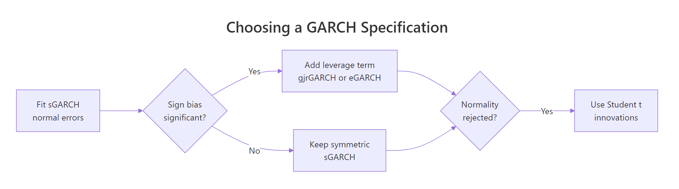
Figure 2: Let the diagnostic tests, not trial and error, pick your specification.
Let us fit the GJR version to the DAX.
spec_gjr <- ugarchspec(
  variance.model     = list(model = "gjrGARCH", garchOrder = c(1, 1)),
  mean.model         = list(armaOrder = c(0, 0), include.mean = TRUE),
  distribution.model = "norm"
)
fit_gjr <- ugarchfit(spec_gjr, dax_ret, solver = "hybrid")

round(fit_gjr@fit$matcoef, 6)
#>         Estimate  Std. Error   t value Pr(>|t|)
#> mu      0.058375    0.021918  2.663338 0.007737
#> omega   0.053992    0.014247  3.789642 0.000151
#> alpha1  0.044245    0.015832  2.794590 0.005197
#> beta1   0.882691    0.023969 36.826536 0.000000
#> gamma1  0.043548    0.023312  1.868090 0.061749
gamma1 is positive at 0.0435, the direction the leverage story predicts, but its p-value is 0.0617, which sits just above the conventional 0.05 threshold. Combined with the Sign Bias test result of 0.1563, the honest reading is that the evidence for asymmetry in this sample is suggestive but not conclusive. Keep that thought, because it changes shortly.
To see what a leverage term actually does, we can compute the news impact curve by hand. This plots tomorrow's variance against the size and sign of today's shock, holding everything else at its long-run level. It is pure arithmetic on the coefficients, so it runs live.
The six coefficients typed into the block below are not new numbers pulled from nowhere. They are the fits of the same two models estimated with Student t shocks rather than normal ones, which is the specification we settle on in the next section: omega 0.021617, alpha 0.079090, beta 0.903588 for the symmetric model, and omega 0.028067, alpha 0.055994, beta 0.890428, gamma 0.058863 for the GJR version. Using the Student t fits here is deliberate, because those are the coefficients we end up trusting.
The blue curve is a clean symmetric parabola: read off the rows for -3 and +3 and both give exactly 1.8611. The red curve is kinked. A 3% drop pushes variance to 2.1730 while a 3% gain pushes it only to 1.6432, about a third less. That is the leverage effect drawn as a picture, and it is why a symmetric model systematically underestimates risk right after a sell-off.
Try it: Using the nic() function above, compute how much more a 2% drop raises tomorrow's variance than a 2% gain under the GJR model, as a ratio.
Click to reveal solution
Explanation: A 2% fall raises tomorrow's variance about 17% more than a 2% rise. The gap widens for larger shocks because the extra gamma term is multiplied by the squared shock.
Which distribution should the shocks follow?
The Adjusted Pearson test rejected normality decisively, so let us find out why. Financial returns are famously fat-tailed: extreme days happen far more often than a bell curve allows.
Part of that fat-tailedness is an illusion created by changing volatility. Mix together calm periods and wild periods and even perfectly normal draws produce a combined distribution with fat tails. A GARCH model should therefore remove some of the excess. Kurtosis measures tail heaviness, and a normal distribution has a kurtosis of 3.
Raw returns have kurtosis 9.27, three times the normal benchmark. But standardizing made it worse, jumping to 15.94, which is the opposite of what the theory predicts. Drop the first 50 observations and it falls to 4.10. Something in the early sample is distorting everything, so let us find it.
There it is. Thirty-five trading days into the sample the DAX fell 9.69% in a single session, at a moment when the model's estimated volatility was only 0.79%. That is a 12-sigma event. Under a normal distribution a 12-sigma move should not occur even once in the lifetime of the universe, yet here is one in a routine 1,859-day sample of a major index.
Excluding the model's warm-up period, kurtosis drops to 4.10, close to but still above the normal benchmark of 3. So the honest summary is: GARCH removes most of the apparent fat-tailedness, and a genuine excess remains. That leftover is what the shock distribution has to handle.
The fix is to let the shocks follow a Student t distribution, which has heavier tails than a normal. Its shape parameter is the degrees of freedom, and lower means fatter.
spec_std <- ugarchspec(
  variance.model     = list(model = "sGARCH", garchOrder = c(1, 1)),
  mean.model         = list(armaOrder = c(0, 0), include.mean = TRUE),
  distribution.model = "std"
)
fit_std <- ugarchfit(spec_std, dax_ret, solver = "hybrid")

round(fit_std@fit$matcoef, 6)
#>         Estimate  Std. Error   t value Pr(>|t|)
#> mu      0.076399    0.018886  4.045289 0.000052
#> omega   0.021617    0.008742  2.472660 0.013411
#> alpha1  0.079090    0.016377  4.829254 0.000001
#> beta1   0.903588    0.020428 44.232208 0.000000
#> shape   6.034057    0.813542  7.417018 0.000000
The estimated shape is 6.03 with a p-value of essentially zero. Six degrees of freedom is a distinctly fat-tailed distribution: a normal is the limiting case as shape goes to infinity, and anything under about 10 is meaningfully heavy-tailed. The data are telling us loudly that they are not normal.
Rather than guess which combination is best, fit a grid and compare with information criteria. AIC and BIC both reward fit and penalise extra parameters, so lower is better, and BIC penalises complexity harder.
grid <- expand.grid(model = c("sGARCH", "gjrGARCH", "eGARCH"),
                    dist  = c("norm", "std", "sstd"), stringsAsFactors = FALSE)

res <- do.call(rbind, lapply(seq_len(nrow(grid)), function(i) {
  s <- ugarchspec(variance.model = list(model = grid$model[i], garchOrder = c(1, 1)),
                  mean.model     = list(armaOrder = c(0, 0), include.mean = TRUE),
                  distribution.model = grid$dist[i])
  f  <- ugarchfit(s, dax_ret, solver = "hybrid")
  ic <- infocriteria(f)
  data.frame(model = grid$model[i], dist = grid$dist[i],
             logLik = round(likelihood(f), 2),
             AIC = round(ic[1], 4), BIC = round(ic[2], 4))
}))
print(res[order(res$BIC), ], row.names = FALSE)
#>     model dist   logLik    AIC    BIC
#>    eGARCH  std -2487.63 2.6828 2.7006
#>    eGARCH sstd -2487.14 2.6833 2.7041
#>    sGARCH  std -2495.26 2.6899 2.7048
#>  gjrGARCH  std -2492.54 2.6880 2.7059
#>    sGARCH sstd -2494.64 2.6903 2.7082
#>  gjrGARCH sstd -2491.94 2.6885 2.7093
#>    eGARCH norm -2589.36 2.7911 2.8060
#>    sGARCH norm -2594.80 2.7959 2.8078
#>  gjrGARCH norm -2592.77 2.7948 2.8097
Look at the shape of that ranking rather than only the winner. Every single model with std or sstd shocks beats every single model with norm shocks. The three normal models occupy the bottom three rows regardless of how sophisticated their variance equation is. Switching distribution improved the log-likelihood by about 100 points; switching from sGARCH to eGARCH while keeping normality improved it by only 5.
One more thing falls out of this table. Earlier, GJR's leverage term looked marginal at p = 0.0617. Refit it with Student t shocks and gamma1 becomes 0.058863 with a p-value of 0.0409, which is significant at the 5% level. The normality assumption had been masking a real asymmetry: forcing thin tails onto fat-tailed data absorbs into the leverage parameter some of what should be tail behaviour.
Try it: Compute the excess kurtosis, meaning kurtosis minus 3, of the standardized residuals after dropping the first 50 warm-up observations. How far from normal is what remains?
Click to reveal solution
Explanation: The raw returns had excess kurtosis of 6.27. After the GARCH model absorbs the volatility clustering, only 1.10 remains. GARCH explained about 82% of the excess tail weight, and the Student t distribution is there to cover the rest.
How do you forecast volatility, and can you trust the forecast?
Everything so far described the past. Forecasting uses the same recursion, pushed forward. For one day ahead there is no guesswork at all, because both inputs are already known.
$$\sigma_{T+1}^2 = \omega + \alpha_1 \varepsilon_T^2 + \beta_1 \sigma_T^2$$
Let us compute it directly using the Student t model's coefficients, along with the final shock and final volatility from that fit.
The model forecasts 1.63% volatility for the next day. Beyond one day we do not know the future shock, so we replace $\varepsilon^2$ with its expected value, which is the variance itself. The recursion then collapses to a single line:
$$\sigma_{T+k}^2 = \omega + (\alpha_1 + \beta_1)\,\sigma_{T+k-1}^2$$
Persistence is now the only thing driving the path.
The forecast starts at 1.63% and decays a little each day toward 1.12%, the long-run level. This is the defining behaviour of a GARCH forecast: it always drifts back to the unconditional volatility, quickly when persistence is low and slowly when it is high. Today's turbulence fades; it does not last forever.
Now let us confirm that rugarch does exactly this.
fc <- ugarchforecast(fit_std, n.ahead = 10)

round(as.numeric(sigma(fc)), 6)
#>  [1] 1.630628 1.623117 1.615702 1.608382 1.601156 1.594024 1.586983 1.580034 1.573176 1.566407

round(as.numeric(fitted(fc)), 6)
#>  [1] 0.076399 0.076399 0.076399 0.076399 0.076399 0.076399 0.076399 0.076399 0.076399 0.076399
The sigma() column is identical to the path we computed by hand, to six decimal places. ugarchforecast() is running the same three lines of arithmetic you just wrote.
Now look at the second output, the forecast of the returns themselves. It is 0.076399 on every single day, a flat line equal to the estimated mean. This is the point readers most often get wrong.
What volatility forecasts are genuinely used for is risk, and risk is usually quoted per year. Convert with the square root of the number of trading days.
Variance grows roughly in proportion to time, so volatility grows with the square root of time, giving the familiar sqrt(252) factor for daily data. The model says the market is currently priced for about 26% annualised volatility against a long-run average near 18%. Those two figures come from the Student t fit; the plain tseries fit from earlier puts the long-run level slightly lower, at 1.04% daily or 16.5% annualised, because the two fits divide the same data differently between the variance equation and the tail of the distribution. That is a statement a risk committee can act on, and it came from three coefficients.
Try it: Suppose a different asset has omega 0.03, alpha 0.10 and beta 0.85, with a one-day-ahead variance forecast of 4.0. Project the volatility five days ahead and compare it with the long-run level.
Click to reveal solution
Explanation: Volatility falls from 2.00 to 1.84 over five days, still far above the long-run 0.77. With persistence of 0.95 the half-life is about 13.5 days, so after only five days most of the shock is still present.
How do you know your forecasts are actually any good?
Everything up to here was in-sample. The model saw all the data before being judged on it, which is not evidence of anything. The real test is a rolling backtest: fit on data up to a point, forecast one day forward, step forward, refit periodically, and score only the forecasts the model never saw the answers to.
ugarchroll() does this. Below it produces 500 genuine one-step-ahead forecasts, refitting every 50 days on a moving window.
roll <- ugarchroll(spec_std, data = dax_ret, n.ahead = 1,
                   forecast.length = 500, refit.every = 50,
                   refit.window = "moving", solver = "hybrid",
                   calculate.VaR = TRUE, VaR.alpha = c(0.01, 0.05),
                   keep.coef = TRUE)

report(roll, type = "fpm")
#>
#> GARCH Roll Mean Forecast Performance Measures
#> ---------------------------------------------
#> Model		: sGARCH
#> No.Refits	: 10
#> No.Forecasts: 500
#>
#>      Stats
#> MSE 1.6870
#> MAE 0.9704
#> DAC 0.5520
MSE and MAE are the average squared and average absolute error of those 500 variance forecasts, and DAC is directional accuracy, which is not informative here because GARCH does not forecast direction in the first place. Error numbers like these mean little on their own anyway. A forecast is only good or bad relative to a sensible alternative, and the obvious alternative is "just use the historical standard deviation and never update it". We can run that comparison live, fitting on all but the last 500 days and rolling the variance recursion forward across them.
GARCH beats the naive constant-variance forecast by about 9% in mean squared error on data it never saw. That is a real improvement, and it is also a modest one. Anyone promising that GARCH transforms volatility forecasting is overselling it. What GARCH reliably does is tell you when risk is elevated, which the constant benchmark can never do.
The sharpest test is Value at Risk. A 1% VaR is a loss level that should be breached on about 1% of days. Count the breaches and you have a direct verdict.
report(roll, type = "VaR", VaR.alpha = 0.01, conf.level = 0.95)
#> VaR Backtest Report
#> ===========================================
#> Model:				sGARCH-std
#> Backtest Length:	500
#>
#> ==========================================
#> alpha:				1%
#> Expected Exceed:	5
#> Actual VaR Exceed:	10
#> Actual %:			2%
#>
#> Unconditional Coverage (Kupiec)
#> Null-Hypothesis:	Correct Exceedances
#> LR.uc Statistic:	3.914
#> LR.uc Critical:		3.841
#> LR.uc p-value:		0.048
#> Reject Null:		YES
#>
#> Conditional Coverage (Christoffersen)
#> Null-Hypothesis:	Correct Exceedances and
#> 					Independence of Failures
#> LR.cc Statistic:	4.323
#> LR.cc p-value:		0.115
#> Reject Null:		NO
Read the two tests together, because they say different things and the combination is the whole story.
Kupiec asks whether the number of breaches is right. Expected 5, observed 10, p-value 0.048, rejected. The model underestimates how far the tail extends.
Christoffersen asks whether the breaches are independent, meaning they do not arrive in clusters. p-value 0.115, not rejected. The breaches are spread out rather than bunched.
Put together: the model gets the timing of risk right and the depth of risk wrong. It knows which weeks are dangerous, since breaches are not clustering. It still underestimates how bad the worst days can be. And you already met the reason, back in the kurtosis section: a 12-sigma day sits in this sample, and no model with only six degrees of freedom of tail was ever going to price that correctly.
Try it: Count VaR breaches yourself. Given the simulated returns below and a constant volatility of 1, the 1% VaR under a normal assumption is qnorm(0.01), about -2.326. Count how many returns fall below it out of 500.
Click to reveal solution
Explanation: Eleven breaches against five expected, a rate of 2.2% instead of 1%. The returns were deliberately drawn from a fat-tailed t distribution while the VaR was computed with a normal quantile. This is exactly the failure the DAX backtest exhibited, reproduced in miniature.
What goes wrong in practice, and should you still use rugarch?
Three mistakes account for most broken GARCH models, and all three are silent.
Mistake one: fitting prices instead of returns. GARCH assumes a stationary series that hovers around a fixed mean. Prices trend, so they do not qualify.
The output is nonsense. Omega comes back as roughly one million because it is trying to describe the variance of index levels, and beta comes back as exactly zero, so the fitted model carries no memory term at all. R also prints a singular information warning alongside that fit, which is how it reports that the estimation is degenerate. Always difference and log first.
Mistake two: forgetting how scaling moves omega. Returns as decimals and returns as percentages are the same data, but the coefficients do not all behave the same way.
Compare with the percent-scale fit: alpha was 0.068377 and beta 0.887741, essentially unchanged. But omega went from 0.047462 to 0.0000047459, smaller by a factor of 10,000, which is 100 squared. Alpha and beta are scale-free ratios; omega carries the units of variance. This is why omega values look wildly different across papers, and why you should never compare omega between two fits without checking the scale first.
Mistake three: a fit that does not converge. If ugarchfit() returns NaN standard errors or an obviously wrong fit, try solver = "hybrid", which is what every rugarch block in this article uses. It falls back through several optimisers instead of giving up on the first failure. If persistence comes back at 0.9999 or above, your model is effectively IGARCH, meaning shocks never decay and there is no finite long-run variance. That is occasionally real, and more often a sign of a structural break sitting in the middle of your sample.
There is one more thing worth knowing before you build anything long-lived on this package.
tsgarch package by the same author. Learn rugarch anyway, because every existing codebase, course and paper uses it, but start new long-lived projects with the successor in mind.The translation is mostly mechanical, with one trap:
| Task | rugarch | tsgarch |
|---|---|---|
| Describe the model | ugarchspec(...) |
garch_modelspec(y, model = "garch", order = c(1,1)) |
| Fit it | ugarchfit(spec, data) |
estimate(spec) |
| Forecast | ugarchforecast(fit, n.ahead = 10) |
predict(fit, h = 10) |
| Backtest | ugarchroll(...) |
tsbacktest(...) |
| Asymmetric model | model = "gjrGARCH" |
model = "gjrgarch" |
The trap is the mean equation. garch_modelspec() has no armaOrder argument at all, only a constant flag. ARMA dynamics moved into a separate package, tsarma. If you are porting a model that relied on rugarch's ARMA mean, that part does not translate directly.
Try it: Predict, without running it, what happens to omega if you fit the same returns divided by 10 rather than 100. Would alpha and beta change?
Click to reveal solution
Dividing returns by 10 divides their variance by 100, so omega should shrink by a factor of 100, from about 0.047462 to about 0.00047462. Alpha and beta would be essentially unchanged, because both are dimensionless ratios describing how variance propagates rather than how large it is.
The general rule: rescaling returns by a factor c rescales omega by c squared and leaves alpha, beta and persistence alone. Every derived quantity that depends only on persistence, such as half-life, is also unaffected.
Practice Exercises
These combine several ideas at once. All three run in your browser.
Exercise 1: A complete workflow on the FTSE
Run the full pipeline on the FTSE index: test for ARCH effects, fit a GARCH(1,1), report persistence, half-life and long-run daily volatility, then forecast five days ahead by hand. Use my_ prefixes so you do not overwrite tutorial variables.
Click to reveal solution
Explanation: The FTSE has clear ARCH effects and very high persistence at 0.9875, giving a 55-day half-life. Notice how flat the five-day forecast is, falling only from 1.170 to 1.156. With persistence that close to 1, forecasts barely move over a week, which is the practical meaning of a long memory.
Exercise 2: Which European market has the longest volatility memory?
EuStockMarkets holds four indices: DAX, SMI, CAC and FTSE. Fit a GARCH(1,1) to each and build a comparison table of alpha, beta, persistence, half-life and long-run daily volatility. Which market forgets a shock fastest?
Click to reveal solution
Explanation: The SMI forgets fastest, with a half-life of 4.5 days, and it has the highest alpha at 0.127 combined with the lowest beta at 0.731, so it reacts sharply to news but does not dwell on it. The FTSE is the opposite: the lowest alpha, the highest beta, and a 55-day memory. Same asset class, same period, and volatility half-lives spanning more than a factor of ten.
Exercise 3: Build a VaR backtest from scratch
Using the DAX model already fitted as g, compute the 1% Value at Risk for each day as qnorm(0.01) * sigma_t + mean(dax_ret), count how many actual returns fell below their VaR, and compare with the 1% you would expect. Does the normal assumption hold up?
Click to reveal solution
Explanation: Thirty breaches where 18.6 were expected, a rate of 1.6% instead of 1%. This mirrors the out-of-sample rugarch backtest almost exactly, and it is the same diagnosis: the GARCH variance dynamics are sound, but pairing them with a normal distribution understates the tail. Rerunning this with a Student t quantile in place of qnorm() moves the count much closer to expectation.
Complete Example
Here is the whole workflow as one reusable function. Give it a price series and it returns a labelled volatility report.
Every line traces back to something built earlier: arch_lm() from the testing section, the recursion from the simulation section, half-life from the interpretation section, the Ljung-Box residual check from the diagnostics section, and the forward recursion from the forecasting section. Swap in EuStockMarkets[, "CAC"] and you get the same report for the French market.
Frequently Asked Questions
How much data do I need to fit a GARCH model?
Maximum likelihood needs a lot of observations to pin down three parameters that describe rare events, and beta in particular is badly estimated in short samples. A practical floor for daily data is around 500 observations, with 1,000 or more preferred, which is why the DAX sample of 1,859 days here is comfortable. Below a few hundred points you will often see beta drift toward 1 or standard errors that swamp the estimates, and the fix is more data rather than a cleverer specification.
Do I need to fit an ARMA model to the returns first?
Test before you assume. Run the Ljung-Box test on the raw returns: if the p-value is large, as it was for the DAX at 0.78, there is no direction to model and a constant mean is correct. If it is small, fit the ARMA mean and the GARCH variance together in one ugarchspec() via armaOrder, rather than fitting ARIMA first and running GARCH on the residuals, because the two-step route understates the standard errors.
My alpha plus beta came out above 1. What went wrong?
Most often nothing is wrong with your code and something is wrong with the sample. A persistence estimate at or above 1 means shocks never fade and there is no finite long-run variance, and the usual cause is a structural break sitting inside the sample, such as a regime change or a merged series from two different assets. Split the sample at the suspected break and refit each half before concluding that the volatility genuinely has infinite memory.
Is GARCH(1,1) enough, or should I try higher orders?
GARCH(1,1) is famously hard to beat on daily financial returns, and higher orders usually buy a fraction of a log-likelihood point for an extra parameter. The horse race in this article makes the same point from the other direction: changing the shock distribution was worth about 100 log-likelihood points, while changing the variance equation was worth about 5. Try (2,1) if the diagnostics on squared standardized residuals still fail, but change the distribution first.
Can I use GARCH to forecast prices or the direction of the market?
No. GARCH forecasts the conditional variance, and the mean forecast it produces is a flat line at the estimated average return, which the forecasting section above shows explicitly. It is used for position sizing, option pricing, Value at Risk and margin setting, all of which need to know how uncertain tomorrow is rather than which way it goes.
Should I start a new project in rugarch or tsgarch?
If you are learning, reading existing code or reproducing published work, use rugarch, because that is what everything is written in. If you are starting a codebase that has to survive several years, use tsgarch, since rugarch's own README says the package will not be updated further and points users to the successor. The one thing that does not carry over cleanly is the ARMA mean equation, which lives in a separate package, tsarma.
Summary

Figure 3: The complete GARCH workflow, from raw returns to an honest out-of-sample verdict.
The parameters and what they tell you:
| Quantity | Formula | DAX value | What it means |
|---|---|---|---|
| alpha | fitted | 0.068 | How hard volatility reacts to yesterday's news |
| beta | fitted | 0.888 | How much of yesterday's volatility carries over |
| omega | fitted | 0.047 | The baseline anchor, and it moves with your data's scale |
| Persistence | alpha + beta | 0.956 | Fraction of a volatility shock surviving one day |
| Half-life | log(0.5)/log(persistence) | 15.4 days | How long until a shock half fades |
| Long-run volatility | sqrt(omega/(1 - persistence)) | 1.04% daily | The level forecasts drift back toward |
| Annualized | daily * sqrt(252) | 16.5% | The same number in the units risk desks quote |
The decisions, and what drives each one:
- Do I need GARCH at all? Ljung-Box on squared returns, plus the ARCH-LM test.
- Symmetric or asymmetric? The Sign Bias test. If it fires, use gjrGARCH or eGARCH.
- Which distribution? The Adjusted Pearson test. For daily equity data the answer is almost always Student t, not normal.
- Is the fit adequate? Ljung-Box on squared standardized residuals should come back large and boring.
- Is it actually useful? Only a rolling out-of-sample backtest can answer that.
And the three things worth remembering above all:
- GARCH forecasts variance, not returns. The mean forecast is a flat line by design.
- Forecasts always mean-revert to the long-run level, at a speed set entirely by persistence.
- The distribution assumption often matters more than the variance equation. On the DAX it was worth roughly twenty times as much log-likelihood.
References
- Bollerslev, T. Generalized Autoregressive Conditional Heteroskedasticity. Journal of Econometrics, 31(3), 307-327 (1986). The paper that introduced GARCH. Link
- Engle, R. F. Autoregressive Conditional Heteroscedasticity with Estimates of the Variance of United Kingdom Inflation. Econometrica, 50(4), 987-1007 (1982). The original ARCH paper, which won the 2003 Nobel Prize. Link
- Galanos, A. rugarch: Univariate GARCH Models. CRAN package documentation and introductory vignette. Link
- Galanos, A. rugarch README, containing the maintenance and migration notice. Link
- Galanos, A. tsgarch: Univariate GARCH Models, the successor package. Link
- Glosten, L. R., Jagannathan, R., and Runkle, D. E. On the Relation between the Expected Value and the Volatility of the Nominal Excess Return on Stocks. Journal of Finance, 48(5), 1779-1801 (1993). The GJR-GARCH model. Link
- Nelson, D. B. Conditional Heteroskedasticity in Asset Returns: A New Approach. Econometrica, 59(2), 347-370 (1991). The EGARCH model. Link
- Perlin, M. S., Mastella, M., Vancin, D. F., and Ramos, H. P. A GARCH Tutorial with R. Revista de Administracao Contemporanea, 25(1) (2021). A peer-reviewed applied walkthrough. Link
- Trapletti, A. and Hornik, K. tseries: Time Series Analysis and Computational Finance. CRAN package documentation. Link
Continue Learning
- ARIMA Models in R covers the mean-equation side of time series modelling. GARCH handles the variance; ARIMA handles the level, and serious models often combine both.
- Test Stationarity in R explains the ADF and KPSS tests. Since GARCH requires a stationary input, this is the check to run before you difference and log your prices.
- Time Series Forecasting in R walks through building and evaluating forecasts more generally, including the accuracy measures used in the backtesting section above.