Benchmark Forecasts in R: Naive, Seasonal Naive, and Drift
A benchmark forecast is a deliberately simple prediction that any real forecasting model has to beat before it earns its keep. R gives you four of them: repeat the last value (naive()), repeat last season (snaive()), extend the straight line (rwf(drift = TRUE)), or use the average of history (meanf()).
Why does every forecast need a benchmark?
Every forecasting project runs into the same question: is this model any good? An error of 70 passengers per month means nothing on its own. It only becomes meaningful next to a reference point, and the reference point is a forecast so simple it fits on one line. Here is that reference on monthly airline passenger counts, scored on two years of data the forecast never saw.
Three things happened there. window() cut the AirPassengers series into a training piece (1949 to 1958) and a test piece (1959 to 1960). snaive() produced 24 monthly forecasts by copying the matching month from the previous year. accuracy() then compared those forecasts against both the data used to build them (the Training set row) and the data held back (the Test set row).
Read the Test set row, because it is the only honest one. On data it had never seen, this one-line forecast missed by about 71 passengers on average, which is 15.5% of the actual value. That number is your floor. Any model you build from here has to come in under it.
If you are new to RMSE, MAE and MAPE, they are three ways of averaging how far the forecasts landed from the actuals, all in the same direction: smaller is better. The forecast accuracy tutorial covers each one in detail, and this page treats them purely as scoreboards.
Try it: Score a plain naive() forecast on the exact same split and see how much worse it is than the seasonal naive 76.99.
Click to reveal solution
Explanation: The naive forecast holds December 1958 flat for two years, so it misses every seasonal peak and trough. Its RMSE of 137.33 is nearly double the seasonal naive score, which tells you the seasonality in this series is real and worth capturing.
What is the naive method, and when is it hard to beat?
The naive method makes one assumption: tomorrow looks like today. Every future value is set equal to the most recent observation, no matter how far ahead you forecast.
In symbols, where $y_T$ is the last observation you have and $h$ is how many periods ahead you want to go:
$$\hat{y}_{T+h|T} = y_T$$
Where:
- $\hat{y}_{T+h|T}$ = the forecast for period $T+h$, made using data up to period $T$
- $y_T$ = the value of the series at the final observed period
- $h$ = the forecast horizon, so $h = 1$ is next month and $h = 12$ is a year out
Before running the function, find the number it will use. The training series ends in December 1958, so the naive forecast is whatever that month recorded.
The training set holds 120 monthly observations, and the last three are October, November and December 1958. December closed at 337 passengers, so that is the only number the naive method cares about.
Now let the function do it. naive() returns a forecast object, and its $mean element holds the point forecasts.
Every forecast is 337, the December 1958 value, repeated for as long as you ask. Plotted, a naive forecast is a horizontal line running off the end of the series.
That sounds too crude to be useful, and on seasonal data it is. On financial and many economic series it is close to unbeatable, because those series genuinely have no memory of where they were: the best guess for tomorrow's price really is today's price. The daily DAX stock index that ships with R makes the point.
We pulled the DAX column out of EuStockMarkets, trained on the first 1600 trading days, and forecast the next 20. The naive forecast is off by 2.12% on average. The mean method, which averages the whole history, is off by 46.42%, because the index climbed steadily: most of the values it averages are far below the level it has now reached.
Anything that behaves like a cumulative running total, prices, exchange rates, inventory levels, tends to reward the naive forecast and punish anything that averages the past.
Try it: The Nile dataset records annual flow of the river Nile from 1871 to 1970. Build a naive forecast for 1961 to 1963 from data up to 1960 and confirm every forecast equals the 1960 flow.
Click to reveal solution
Explanation: The 1960 flow was 815, so all three forecasts are 815. The horizon changes nothing, which is exactly what the naive formula says.
What is the seasonal naive method, and why does it own seasonal data?
Airline passengers do not wander randomly. Every July is busy and every November is quiet, year after year. The naive method throws all of that away by holding one number flat. The seasonal naive method keeps it by copying the value from the same season one cycle back.
For a monthly series the cycle length is $m = 12$, so the forecast for next March is last March, and the forecast for March two years out is still last March (the most recent one available).
$$\hat{y}_{T+h|T} = y_{T+h-m(k+1)}$$
Where:
- $m$ = the number of periods in one seasonal cycle (12 for monthly data, 4 for quarterly)
- $k$ = the integer part of $(h-1)/m$, which is just how many complete cycles the horizon spans
- $y_{T+h-m(k+1)}$ = the observation from the same season in the most recent complete cycle
The formula looks fussy but the behaviour is simple. Print the final year of the training data and you have already printed the forecast.
That is the calendar year 1958: a January of 340, a summer peak of 505 in August, a November trough of 310. The seasonal naive method predicts 1959 will look exactly like this.
The first 12 forecasts are the 1958 vector, value for value. Ask for 24 months and the second year is the same 12 numbers again, because 1958 is still the most recent complete cycle.
You never told snaive() that the cycle is 12 months long. It reads $m$ from the series itself: a ts object carries a frequency attribute, and AirPassengers has frequency = 12. This matters when you move to your own data. If you hand snaive() a plain numeric vector, or a ts built without setting frequency, then $m = 1$ and the seasonal naive forecast is identical to the naive forecast. Check frequency(y) before you trust an snaive() result.
This is why the seasonal naive score of 76.99 was so much better than the naive score of 137.33 earlier. Copying the seasonal shape captures most of what makes this series move.
Try it: Show that the seasonal naive forecast repeats itself with a 12-month period by comparing the forecast at horizons 1 and 13, and at horizons 2 and 14.
Click to reveal solution
Explanation: Horizon 13 is January 1960 and horizon 1 is January 1959, and both copy January 1958. The forecast is periodic with period 12 forever.
What is the drift method, and how does it extend a trend?
The naive forecast is a flat line. The drift method takes that flat line and tilts it, so the forecast keeps moving in the direction the series has been moving. The tilt is not fitted by regression: it is simply the average change per period across the whole history.
$$\hat{y}_{T+h|T} = y_T + h\left(\frac{y_T - y_1}{T-1}\right)$$
Where:
- $y_1$ = the first observation in the series
- $y_T$ = the last observation
- $T$ = the number of observations
- $\frac{y_T - y_1}{T-1}$ = the average change per period, which is the drift
The fraction is worth staring at. Total change divided by number of steps is the slope of the straight line joining the first point to the last point. Drift extends that line, nothing more.
The series started at 112 passengers in January 1949 and ended at 337 in December 1958, across 119 steps, so it gained an average of 1.89 passengers per month. Now compare the package output against the formula applied by hand.
The two lines agree exactly. rwf() stands for random walk forecast, and adding drift = TRUE turns the flat naive line into a sloped one. The first forecast is 337 plus one step of drift, the second is 337 plus two steps, and so on.
The catch is in the formula: only $y_1$ and $y_T$ appear. Everything between them is ignored. If either endpoint happens to be an unusual month, the whole slope tips with it.
Try it: Compute the drift slope for the Nile training series by hand, then check it against rwf().
Click to reveal solution
Explanation: The slope is negative, so each forecast sits 3.427 below the one before it. Flow in 1871 was much higher than in 1960, and drift reads that as a steady decline even though the real series dropped once around 1899 and then stayed flat.
What is the mean method, and when is the average the best guess?
The mean method ignores order completely. It averages every observation in the training data and forecasts that single number forever.
$$\hat{y}_{T+h|T} = \bar{y} = \frac{y_1 + y_2 + \dots + y_T}{T}$$
That sounds even cruder than naive, and on trending or seasonal data it is. On a series that wobbles around a stable level, it is the strongest of the four, because averaging cancels out noise that the naive method treats as signal. The Nile flow record is exactly that kind of series.
meanf() forecast every year from 1961 to 1970 as 924.3, the average of the previous 90 years. On the held-out decade it scored an MAE of 118 against the naive method's 128, so the average was the better guess.
The reason is that the Nile reverts. A high-flow year is usually followed by a return toward the long-run level, so anchoring on a single recent year (which is all naive does) inherits that year's noise. The DAX index never reverts, which is why the same comparison went the other way there.
Try it: Run the mean method on the AirPassengers training set and score it against the same test set used earlier. It should lose badly.
Click to reveal solution
Explanation: The average across 1949 to 1958 includes the low early years, so it sits far below the 1959 to 1960 level it is asked to predict. On a trending series the mean method is the worst of the four benchmarks.
How do you fit and compare all four benchmarks at once?
You do not have to choose a benchmark by eye. Fit all four, score them on the same held-out data, and read the table. The whole comparison is a list of forecasts and one sapply().
The list holds four forecast objects built the same way. sapply() walks the list, pulls the Test set row out of each accuracy() call, and t() flips the result so each method gets a row.
A fourth metric joins the table here. MASE, the mean absolute scaled error, divides the test-set error by the average error a naive forecast made inside the training data (the seasonal naive version of it when the series is seasonal). That division cancels the units, so a MASE of 2.49 reads as "about two and a half times the in-sample naive error" and can be compared across series measured in completely different things. Like the other three, smaller is better.
Seasonal naive wins on every metric, drift comes second, and the mean method is a distant last. That ranking tells you what this series is made of: seasonality dominates, a mild trend sits underneath it, and there is no stable level for the mean method to settle on.
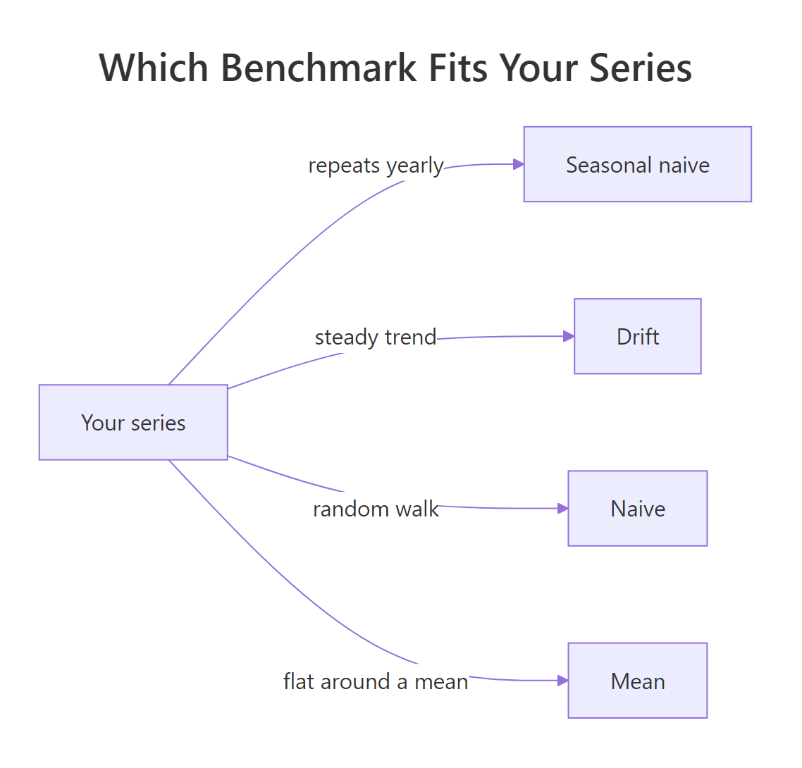
Figure 1: Match the benchmark to the shape of your series.
Numbers rank the methods, but a plot shows you why. Drawing all four forecast paths over the actual data makes each method's assumption visible.
The blue seasonal naive line is the only one with the right shape, though it sits below the actual 1959 and 1960 data because it cannot grow. Red (naive) and green (drift) are straight lines, one flat and one tilted upward. Orange (mean) sits far below everything, exactly as its 44% error suggested.
Try it: Repeat the bake-off on USAccDeaths, monthly accidental deaths in the USA from 1973 to 1978. Train through 1977 and test on the 12 months of 1978.
Click to reveal solution
Explanation: Seasonal naive is nearly three times more accurate than anything else, because deaths peak every summer. The other three all score around 950 since none of them can represent a seasonal pattern.
Why do benchmark prediction intervals fan out, and how wide should they be?
A point forecast is a single number, and a single number is always wrong. What you actually want is a range. Each of these methods comes with prediction intervals, and reading how those intervals grow tells you a lot about the method.
Start with the seasonal naive intervals for the first four months.
sn_fc$lower and sn_fc$upper are matrices with one column per confidence level, 80% first and 95% second, which is why we asked for column 2. The January forecast of 340 comes with a 95% range of 276 to 404.
Notice the width is identical for all four rows, about 127 passengers. That is not a bug. Every one of those forecasts copies an observation from the same single year of data, so each carries exactly the same amount of uncertainty.
The width only jumps when the horizon crosses into a second seasonal cycle.
The interval at horizon 13 is 1.414 times wider than at horizon 1, and 1.414 is the square root of 2. The measured ratio matches the formula exactly, and here is the formula it matches. Each method has an expression for the forecast standard deviation $\hat{\sigma}_h$ at horizon $h$, built from $\hat{\sigma}$, the standard deviation of the errors the method made inside the training data:
$$\text{Naive: } \hat{\sigma}_h = \hat{\sigma}\sqrt{h} \qquad \text{Seasonal naive: } \hat{\sigma}_h = \hat{\sigma}\sqrt{k+1}$$
$$\text{Drift: } \hat{\sigma}_h = \hat{\sigma}\sqrt{h\left(1 + \frac{h}{T-1}\right)} \qquad \text{Mean: } \hat{\sigma}_h = \hat{\sigma}\sqrt{1 + \frac{1}{T}}$$
Where $k$ is again the number of complete seasonal cycles inside the horizon, so $k = 0$ for the first year of monthly forecasts and $k = 1$ for the second. Two years out means $\sqrt{2}$ times the uncertainty, which is the 1.414 we just measured.
The interval itself is then the point forecast plus or minus a multiplier times $\hat{\sigma}_h$: 1.28 for an 80% interval and 1.96 for a 95% interval, the usual normal-distribution numbers.
Try it: Check the naive square root rule directly. Using nv_fc from earlier, confirm the 95% interval at horizon 4 is exactly twice as wide as at horizon 1.
Click to reveal solution
Explanation: For the naive method the uncertainty grows with the square root of the horizon, so four steps out is exactly twice as uncertain as one step out. Growing intervals are the honest way of saying that the far future is harder to call.
How do you prove a real model beats the benchmark?
A benchmark does two jobs. It sets the score to beat, and its residuals tell you whether there is anything left worth modelling.
Residuals are what the forecast missed inside the training data, one number per period. If a method has extracted everything predictable, the residuals should look like random noise with no pattern. The Ljung-Box test formalises that: a small p-value means the residuals are still correlated with their own past, so predictable structure remains.
The p-value is essentially zero, so the residuals are strongly autocorrelated. checkresiduals() also draws a residual time plot, a histogram, and an ACF panel. ACF is short for autocorrelation function, and that panel plots how strongly the residuals still correlate with their own values 1, 2, 3 and more periods earlier. Here those bars decay slowly instead of dropping to near zero, and the residual mean sits well above zero, which is the upward trend the seasonal naive method cannot represent. A better model definitely exists for this series.
Now run the same check on the DAX naive forecast for contrast.
A p-value of 0.987 means there is no detectable autocorrelation left. The naive method has already captured everything this series has to offer, and a more complex model would be fitting noise.
So the AirPassengers series has room to improve. Two standard models now get scored on the same 24-month test window: ets() fits an exponential smoothing model and auto.arima() fits an ARIMA model, and both search their own family of candidates and return the best-fitting one, so neither needs any settings from you here.
Both beat the seasonal naive score of 76.99, so the residual test was right that something was left on the table. Look at the margin though: exponential smoothing improves RMSE by about 6% and ARIMA by about 4%. That is a real gain, and it is also much smaller than most people expect from replacing a one-line forecast with a fitted model.
That margin is the number to take to whoever is paying for the work. Six percent may be worth a maintained model, or it may not be worth the extra failure modes, and only a benchmark lets you have that conversation with numbers.
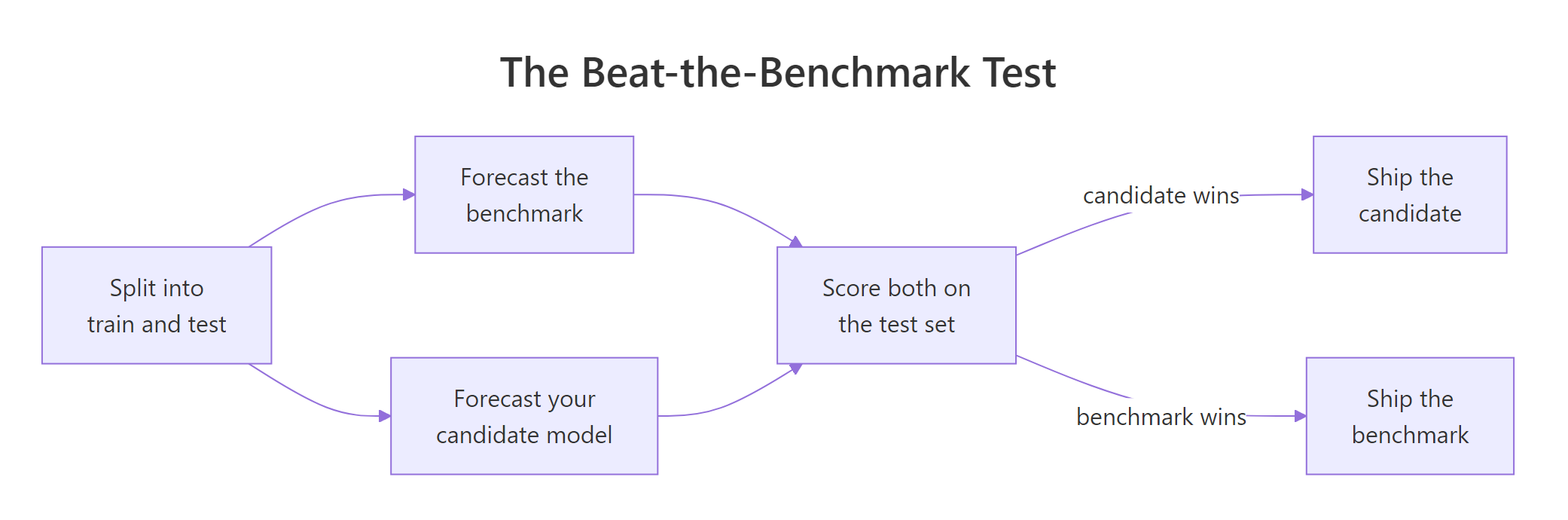
Figure 2: Fit the benchmark and the candidate on the same training data, score both on the same held-out test set, then ship whichever wins.
Try it: Run the beat-the-benchmark test on USAccDeaths. Fit ets() on ua_train, forecast 12 months, and compare it against the seasonal naive score.
Click to reveal solution
Explanation: ETS improves RMSE by about 15%, a clearer win than on AirPassengers. Both MASE values are below 1, meaning both forecasts are more accurate on the test set than an in-sample seasonal naive forecast was on the training data.
Complete Example: the same four benchmarks in fable
The forecast package works with base R ts objects. The newer fable package works with tsibbles, keeps every model in a single table, and scales to thousands of series at once. The benchmarks are the same, only the spelling changes: NAIVE(), SNAIVE(), RW(y ~ drift()) and MEAN().
Start by converting AirPassengers into a tsibble, a data frame that knows which column is time. The |> in the next few blocks is base R's pipe: x |> f() means exactly f(x), and chaining it keeps a long sequence of steps readable top to bottom.
The [1M] tag confirms a monthly index. Now fit all four benchmarks plus an ETS model in one model() call, forecast 24 months, and score everything against the full series.
filter_index(~ "1958 Dec") keeps everything up to December 1958, matching the window() split from the start of this page. Each argument to model() becomes a column of fitted models, forecast() produces all five forecasts at once, and accuracy() scores them against the actual values it finds in ap.
The ranking is identical to the forecast package table, down to the decimals: ETS at 72.5, seasonal naive at 77.0, then drift, naive and mean. Two different packages, two different object systems, same answer. If you want the tidy workflow in depth, the fable and tsibble tutorial covers the full pipeline.
Practice Exercises
Exercise 1: Find the best benchmark for UK road deaths
UKDriverDeaths records monthly drivers killed or seriously injured in the UK from 1969 to 1984. Train on everything up to December 1982, forecast the 24 months of 1983 and 1984, and score all four benchmarks. Which one wins, and by how much?
Click to reveal solution
Explanation: Seasonal naive wins with an RMSE of 325.27, less than half the naive score. Every method still has a large error because seat belt legislation took effect in January 1983 and cut deaths sharply, a change no benchmark could have anticipated from past data alone.
Exercise 2: Rebuild the drift forecast from scratch
Without calling rwf(), compute all 24 drift forecasts for the AirPassengers training set using only the formula, then prove your vector matches the package output exactly.
Click to reveal solution
Explanation: all.equal() returns TRUE, so the hand-built vector is identical to the package output. The drift method has no hidden estimation step: the entire model is one subtraction, one division and one multiplication.
Exercise 3: Decide whether ETS is worth it for UK road deaths
Using the same ex_uk_train and ex_uk_test split from Exercise 1, fit an ETS model, score it against the seasonal naive benchmark, and decide which one you would ship.
Click to reveal solution
Explanation: The benchmark wins. Seasonal naive scores 325.27 against the ETS score of 336.36, so the fitted model is worse on the data that matters. Ship the benchmark here, and note that both MASE values above 2 signal a structural break in the test period rather than a modelling failure.
Frequently asked questions
Is the naive method really used in practice?
Yes, and more often than most tutorials admit. Financial forecasting treats the naive forecast as the default because prices behave like random walks, and short-horizon operational forecasts frequently use last week's value as the plan. It is also the standard baseline in forecasting competitions, so any published accuracy claim is implicitly measured against it.
Should the benchmark be fitted on the training set only?
Always. If your benchmark sees the test data, its score is optimistic and the comparison is meaningless. Split first, fit both the benchmark and the candidate model on the training piece, and score both on the same untouched test piece. That is exactly what window() and the Test set row of accuracy() are enforcing on this page.
What is the difference between NAIVE(y ~ drift()) and RW(y ~ drift())?
Nothing. In fable, NAIVE() is an alias for RW() with no drift term, and both accept a drift() special, so RW(y ~ drift()) and NAIVE(y ~ drift()) fit the same random walk with drift model. Writing RW(y ~ drift()) is the clearer choice because the name says random walk, which is what a drift model is.
Why is my MASE above 1 even for a seasonal naive forecast?
Because MASE is scaled by the in-sample naive error, a value above 1 just means the test period was harder than the training period. That happens whenever the series grows away from its old level or hits a structural break, and it is not a sign that you fitted the benchmark wrongly. On this page the seasonal naive MASE is 2.49 because passenger numbers in 1959 and 1960 were far above anything in the training years.
Which benchmark should I report in a paper or a stakeholder deck?
Report the seasonal naive method if your data has a seasonal cycle and the plain naive method if it does not. Those two are the conventional baselines in the forecasting literature, so readers can compare your numbers with published results. Adding drift and mean costs one line each and shows you checked rather than assumed.
Summary
Benchmarks turn an unreadable error number into a decision. All four are one-liners, all four run before you model anything, and the winner tells you what your series is made of.
| Method | What it forecasts | R call | Best for | Fails when |
|---|---|---|---|---|
| Naive | The last observed value, repeated | naive(y, h) |
Random walks, prices, short horizons | The series is seasonal or trending |
| Seasonal naive | The same season one cycle back | snaive(y, h) |
Any series with a repeating cycle | The series also trends up or down |
| Drift | Last value plus the average change | rwf(y, h, drift = TRUE) |
Steady trends with no seasonality | Either endpoint is an outlier |
| Mean | The average of all history | meanf(y, h) |
Series that revert to a stable level | The series trends or has seasonality |
The takeaways in one glance:
- A benchmark is the floor your model must clear, so fit it before anything complex.
- Naive and mean are opposites: one assumes the series has no memory, the other assumes it has nothing but memory.
- Seasonal naive is the default baseline for seasonal data, and it is often close to a fitted model's accuracy.
- Drift is defined entirely by the first and last observations, which makes it fast and fragile.
- Prediction intervals fan out with the square root of the horizon, and the seasonal naive width jumps only when the horizon crosses a full cycle.
- If a benchmark's residuals pass the Ljung-Box test, ship the benchmark and move on.
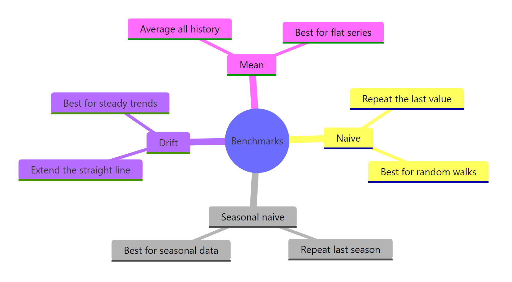
Figure 3: The four benchmark forecasts at a glance.
References
- Hyndman, R.J. & Athanasopoulos, G. - Forecasting: Principles and Practice (3rd ed), "Some simple forecasting methods". Link
- Hyndman, R.J. & Athanasopoulos, G. - Forecasting: Principles and Practice (3rd ed), "Prediction intervals", source of the sigma formulas. Link
- Hyndman, R.J. & Athanasopoulos, G. - Forecasting: Principles and Practice (3rd ed), "Evaluating forecast accuracy". Link
- Hyndman, R.J. - "Benchmarks for forecasting", on which baselines to report. Link
- fable package -
RW()random walk models reference, covering NAIVE, SNAIVE and drift. Link - forecast package -
naive(),snaive()andrwf()reference. Link - R documentation - the
AirPassengersdataset. Link - forecast package on CRAN. Link
Continue Learning
- Forecast Accuracy in R - what RMSE, MAE, MAPE and MASE actually measure, and which to trust.
- Time Series Cross-Validation in R - score benchmarks over many origins instead of one split.
- fable and tsibble in R - the tidy forecasting workflow used in the complete example above.