MSTL in R: Decompose Multiple Seasonalities
MSTL (Multiple Seasonal-Trend decomposition using Loess) splits a series that repeats on more than one clock, say a daily rhythm and a weekly rhythm, into a trend, one seasonal component per period, and a remainder. A single call to mstl() in the forecast package does the whole job. This tutorial builds the idea from scratch on real half-hourly electricity demand, and every code block on this page runs in your browser.
What does a series with two seasonal cycles look like?
Electricity demand climbs every morning and falls every night, and that is one cycle. It also sags every weekend, which is a second cycle sitting on top of the first. Data recorded every half hour therefore repeats every 48 observations and again every 336. The taylor series that ships with the forecast package is exactly that, and one function separates both rhythms.
Read the first row across. At the very first half hour of the series, demand was 22,262 megawatts. The underlying level (Trend) sat at 30,213. Being the middle of the night pulled it down by 5,816 (Seasonal48), the day of the week pulled it down another 1,768 (Seasonal336), and 368 megawatts of unexplained wobble was left over (Remainder).
That is the whole promise of MSTL. Instead of one seasonal column, you get one seasonal column for each cycle you declare, named after its period length.
The data itself is half-hourly electricity demand for England and Wales, starting midnight on Monday 5 June 2000 and running for twelve weeks. Let us look at its shape before going further.
Four thousand and thirty two readings is twelve weeks of half hours (48 x 7 x 12). The msts attribute is the key line: this series already carries two seasonal periods, 48 and 336, rather than the single frequency a plain ts object holds.
Both rhythms are visible without any modelling. Average the series by position in the day, and then again by day of the week. Both patterns fall straight out.
tod labels each reading with its slot inside the day (slot 1 is midnight, slot 13 is 06:00, slot 21 is 10:00, slot 37 is 18:00, slot 48 is 23:30). dow labels each reading with its day, where 1 is Monday because the series starts on a Monday.
The day profile swings from about 24,000 megawatts at midnight to 34,660 at ten in the morning. The week profile is flat from Monday to Friday near 31,000 and then drops to 25,233 on Sunday. Two separate, real, repeating patterns.
Here is the thing that makes MSTL necessary rather than merely convenient. If you hand this series to ordinary stl() and tell it only about the daily cycle, the weekly cycle does not disappear. It ends up inside the components you did ask for.
Two helpers from the forecast package make that visible: trendcycle() pulls the trend column out of a fitted decomposition, and remainder() pulls the leftovers.
The single-season trend swings between 24,125 and 32,391, a range of more than 8,000 megawatts, in a series whose real level barely moves. The MSTL trend, which knows about the weekly cycle, only moves between 28,175 and 30,213.
The final line explains why. That wobbly trend correlates 0.891 with the weekly component MSTL extracted. The undeclared weekly cycle was absorbed into the trend, so most of what looks like a change in the underlying level is really the weekend coming round again.
The leftovers tell the same story. Autocorrelation at lag 336 asks "does this series look like itself one week ago", and for a clean remainder the answer should be close to zero.
acf() returns lag 0 first, so the value for lag 336 sits at index 337. The single-season remainder is 0.861 correlated with itself a week earlier, which is an enormous amount of structure to leave in a component that is supposed to be noise. The MSTL remainder scores -0.053, which is what noise looks like.
Try it: The block below shows the day-of-week averages of the single-season remainder, where Monday and the weekend stick out. Compute the same averages for the MSTL remainder stored in fit and confirm the weekday pattern is gone.
Click to reveal solution
Explanation: The single-season remainder still carries a Monday spike of +433 and a weekend dip near -280, because the weekly cycle had nowhere else to go. Once the weekly period is declared, those averages collapse to a few tens of megawatts on a series that averages 30,000.
How do you tell R that a series has more than one season?
A plain ts object stores exactly one number for seasonality, its frequency. That is why stl() can only ever remove one cycle. The forecast package adds a class called msts (multiple seasonal time series) that stores a whole vector of periods instead.
You build one with msts(), passing the raw numbers and the periods you want recorded.
The object still is a ts underneath, so everything that works on a time series keeps working. The extra msts attribute is what mstl() reads to decide how many seasonal components to carve out.
Note that frequency() reports only the longest period, 336. That is a compatibility fallback for functions that expect a single number, and it is a good reason to check attributes(x)$msts rather than frequency(x) when you want to know what a series actually declares.
Choosing the periods is arithmetic, not guesswork. A period is how many observations pass before the pattern repeats.
| Data recorded | Daily cycle | Weekly cycle | Yearly cycle |
|---|---|---|---|
| Every hour | 24 | 168 | 8766 |
| Every half hour | 48 | 336 | 17532 |
| Every 15 minutes | 96 | 672 | 35064 |
| Every day | not applicable | 7 | 365.25 |
| Every week | not applicable | not applicable | 52.18 |
Two of those numbers are not whole. Daily data does not repeat every 365 days, it repeats every 365.25 days on average, and msts() accepts the fraction happily.
This is three years of made-up daily sales. A slow upward drift runs underneath a weekly shopping rhythm plus a yearly season, with noise on top. The component names come straight from the periods, so a fractional period gives you a column called Seasonal365.25.
Try it: The hourly series below has a daily shape plus a weekend bump. The starter declares only the daily cycle. Declare both the daily and the weekly cycle, then print the component names.
Click to reveal solution
Explanation: Hourly data repeats every 24 observations daily and every 24 x 7 = 168 observations weekly. Notice that asking for a single period gives NULL for the msts attribute: with one period there is nothing multiple about it, so the object stays an ordinary ts.
How does mstl() actually work under the hood?
MSTL does not invent new mathematics. It runs ordinary stl() several times in a loop, peeling off one seasonal pattern per pass, and keeps refining. stl() itself estimates each piece with loess, a smoother that fits a small local regression through the points nearest each time index. That loess step is the L in both STL and MSTL. The model MSTL fits is additive:
$$y_t = T_t + \sum_{i=1}^{k} S_t^{(i)} + R_t$$
Where:
- $y_t$ = the observed value at time $t$
- $T_t$ = the trend, the slow-moving level
- $S_t^{(i)}$ = the seasonal component for the $i$-th declared period
- $k$ = how many periods you declared
- $R_t$ = the remainder, whatever none of the above explains
The loop that estimates those pieces is short enough to say in five steps.
- Sort the declared periods from shortest to longest, and start every seasonal component at zero.
- Take the current de-seasonalised series and add back the seasonal component you are about to re-estimate.
- Run
stl()on that series at this period, and keep its seasonal output as the new estimate. - Subtract the new estimate and move to the next period.
- Repeat the whole sweep (twice by default), then take the trend from the last
stl()fit and call the leftovers the remainder.
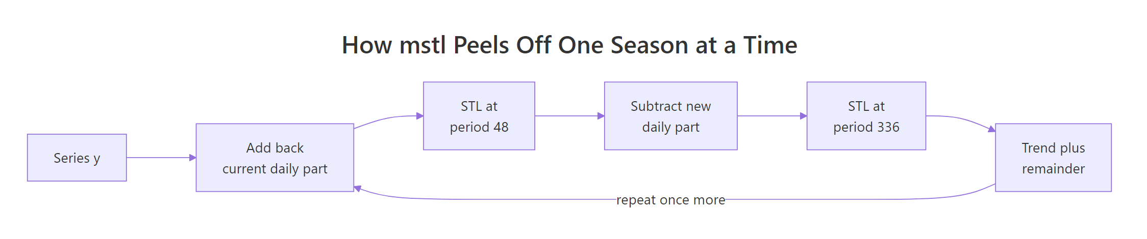
Figure 1: The mstl backfitting loop peels off the shortest season first, then the next, then sweeps again.
Statisticians call this pattern backfitting: each component is re-estimated while holding the others fixed, and the estimates settle down after a sweep or two. The reason it needs sweeps at all is that the first daily estimate is contaminated by the weekly pattern still sitting in the data, so once the weekly part is removed the daily part deserves another look.
You do not have to take that description on faith. The loop is short enough to write out with plain stl() calls and check against the real thing.
Both differences are exactly zero, so those thirteen lines are mstl(). The windows vector holds the seasonal smoothing windows the function uses by default, which the next section unpacks.
Two behaviours are worth knowing before you trust the function on other data. If you pass a plain ts instead of an msts, there is only one period to estimate, so the sweep count drops to one and you get ordinary STL. If the series has no seasonality at all, mstl() skips STL entirely and fits the trend with supsmu(), a general purpose scatterplot smoother.
Try it: The default is two sweeps. Refit taylor with iterate = 1 and measure how far the daily component moves compared with the two-sweep default.
Click to reveal solution
Explanation: The second sweep moves the daily component by up to 552 megawatts and the weekly component by up to 192. On a series with a daily swing of roughly 14,000 megawatts that is a small correction, which is exactly why two sweeps is enough for most data.
How do you read the components, and do they add back up?
The object mstl() returns is a matrix with one column per component. Because the model is a sum, those columns must reconstruct the data exactly. Checking that is the fastest sanity test there is.
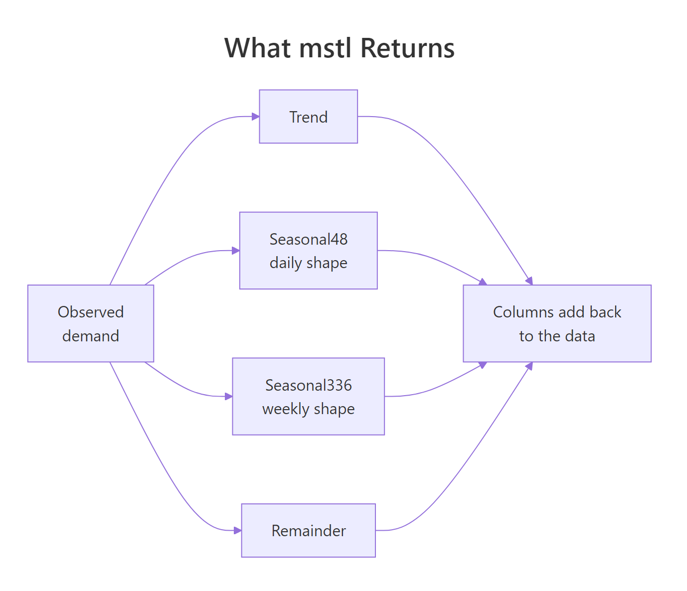
Figure 2: mstl returns one trend, one seasonal column for each declared period, plus a remainder that all add back to the data.
Converting to a data frame with as.data.frame() makes the columns easy to grab by name. The reconstruction matches the original data to within floating point dust, which confirms nothing was lost.
The standard deviations rank the components by size. The daily cycle (4,790) is by far the biggest source of variation, the weekly cycle (2,733) is a bit over half as large, the trend (604) barely moves across twelve weeks, and the remainder (307) is small. That ranking is the summary a stakeholder actually wants: this series is mostly a daily rhythm with a strong weekend effect and almost no underlying growth.
The built-in plot method draws all of it as stacked panels.
Each panel shares the same time axis, so you can line up a spike in the data with the component responsible for it. The grey bars on the right of a forecast-package decomposition plot show the relative scale of each panel, so a tall bar means a small component stretched to fill its panel.
Numbers beat pictures when you need a specific answer, so it helps to fold each seasonal column back into its own shape. Reshaping Seasonal48 into a matrix with 48 rows puts every day in its own column, and averaging across rows gives the typical day.
The daily shape says midnight runs 5,580 megawatts below the day's level, 06:00 is the lowest of the five slots printed here, and mid morning runs about 5,000 above it. Slot 24 is the peak of the whole day, which is 11:30.
The weekly shape says Tuesday through Thursday sit about 1,700 megawatts above the weekly average, Saturday sits 3,115 below, and Sunday 4,324 below. Those two shapes together are the seasonal story of the series in eight numbers.
Subtracting both seasonal columns leaves the seasonally adjusted series, which is what you plot when someone asks whether demand is really rising or just following the calendar.
Raw demand ranges over 20,000 megawatts. Once the daily and weekly calendar effects are removed, the same twelve weeks vary by less than 4,000. Almost all of that 20,000 megawatt spread was the time of day and the day of the week, not any real movement in underlying demand.
Try it: The peak of the daily shape is slot 24. Find the trough slot instead, and report how far below the day's level it sits.
Click to reveal solution
Explanation: Slot 10 is 04:30, and demand there runs 7,862 megawatts below the daily level. Compared with the 11:30 peak of +5,551, the working day moves demand by more than 13,000 megawatts from bottom to top.
How do you tune s.window, iterate, and lambda?
Three arguments cover almost every adjustment you will ever make. The most important is s.window, which controls how quickly a seasonal shape is allowed to change from one cycle to the next.
A small window lets the daily shape evolve week by week. A large window forces it to stay nearly identical, and the special value "periodic" freezes it completely. The default is a vector, paired with the sorted periods.
The default s.window is 7 + 4 * seq_len(6), which is the vector 11, 15, 19, 23, 27, 31. The shortest period gets 11, the next gets 15, and so on, so shorter cycles are allowed to drift more freely than long ones.
Slot 19 is 09:00. Under the default, the 09:00 seasonal effect wanders with a standard deviation of 170 megawatts across the 84 days in the series, which means the morning ramp really does look slightly different from week to week. Under "periodic" that standard deviation is exactly zero, because every day is forced to share one shape.
| Situation | What to do with s.window |
|---|---|
| Short series, or a shape you believe is stable | "periodic" or a large odd number |
| Seasonal shape clearly evolving (new tariffs, new store hours) | Small odd number, 7 to 15 |
| Noisy series where the seasonal estimate looks jittery | Increase the window until it steadies |
| Different periods needing different treatment | Pass a vector, one value per period |
The second argument is iterate, the number of sweeps through the periods, which defaults to 2 and rarely needs changing. The third is lambda, which applies a Box-Cox transformation before decomposing. Reach for it when the seasonal swings grow as the level grows, which is the signature of a multiplicative series.
With lambda = "auto" the function picks a transformation parameter (here -0.123, close to a log) and decomposes the transformed series. Watch the scales in that output. The Data column stays in megawatts while every other column lives on the transformed scale, so the columns no longer add up to the data and the seasonal sizes are no longer readable in the original units.
That is the trade. A Box-Cox decomposition is the right call when seasonal amplitude scales with the level, and the price is that you must back-transform before interpreting component magnitudes.
Try it: The default weekly window is 15. Refit with a very wide weekly window, s.window = c(11, 501), and check how much the weekly shape is still allowed to drift.
Click to reveal solution
Explanation: A window of 501 is far longer than the twelve weeks available, so the weekly shape is effectively frozen and its drift collapses to zero, the same as "periodic". The default window of 15 allowed a modest 32.68 megawatts of week-to-week movement.
How do you check the decomposition actually worked?
A decomposition always returns something. Two checks tell you whether that something is any good, and both take one line each.
The first is the remainder autocorrelation at each seasonal lag, which you already met in the opening section. A large positive value at lag $m$ means a cycle of length $m$ is still sitting in the leftovers.
The single-season fit leaves 0.291 at the daily lag and 0.861 at the weekly lag. The MSTL fit cuts those to 0.119 and -0.053. Declaring the weekly period improved the daily lag too, which is what the backfitting loop is for: removing one cycle makes the other easier to estimate.
The second check is seasonal strength, a number between 0 and 1 that says how much of the non-trend variation a given seasonal component accounts for.
$$F_S = \max\left(0,\; 1 - \frac{\operatorname{Var}(R_t)}{\operatorname{Var}(S_t + R_t)}\right)$$
Where:
- $F_S$ = the strength of that seasonal component
- $S_t$ = the seasonal component being scored
- $R_t$ = the remainder
- $\operatorname{Var}$ = variance across the whole series
If the seasonal component is pure noise, the two variances match and the strength is 0. If the seasonal component dwarfs the remainder, the ratio goes to zero and the strength approaches 1.
Both scores sit above 0.98, which is about as seasonal as real data ever gets. Electricity demand is close to a clockwork process, so this is believable rather than suspicious. Anything above roughly 0.6 counts as strongly seasonal, and anything below 0.3 usually means the period is not worth declaring.
Try it: The same formula scores the trend if you put $T_t$ where $S_t$ was. Compute the trend strength of taylor and compare it with the daily seasonal strength.
Click to reveal solution
Explanation: The trend scores 0.809, which sounds impressive until you recall that this trend only moves 2,000 megawatts across twelve weeks while the daily cycle moves 14,000. Strength measures how cleanly a component stands out from the remainder, never how big it is. Use strength to decide whether a component is real, and the standard deviations from earlier to decide whether it is worth talking about.
How do you decompose multiple seasonality the tidyverts way?
The forecast package is not the only route. The newer tidyverts stack (tsibble, fabletools, feasts) does multi-seasonal STL through a model formula, which fits better when your data already lives in a tsibble.
Instead of declaring periods on the object, you declare them in the formula with one season() term per cycle.
vic_elec is half-hourly electricity demand for Victoria, Australia. The filter above narrows it to January 2014. The result of components() is a dable, a decomposition table, which is a tsibble carrying one column per component plus the ready-made season_adjust column.
The header line spells out the model being fitted, Demand = trend + season_48 + season_336 + remainder, which is the same additive equation from earlier. Adding robust = TRUE tells the loess fits to downweight outliers, which matters for demand data punctuated by heatwaves.
Do the two routes agree? Run both on identical data and correlate the components.
The daily components agree closely at 0.969. The weekly components agree less, at 0.769, because the two implementations pick different default windows and this run also turned on robust fitting. Neither is wrong: they are two reasonable smoothers disagreeing about how much of a January weekend is calendar and how much is weather.
| Task | forecast package | tidyverts |
|---|---|---|
| Declare periods | msts(x, seasonal.periods = c(48, 336)) |
season(period = 48) + season(period = 336) |
| Fit | mstl(x) |
model(STL(y ~ ...)) |
| Get components | the returned matrix | components() |
| Seasonally adjusted | subtract the seasonal columns | the season_adjust column |
| Robust to outliers | pass robust = TRUE through to stl |
STL(..., robust = TRUE) |
Try it: The formula above used raw observation counts. Rewrite it with the human readable period strings "1 day" and "1 week", then print the component names.
Click to reveal solution
Explanation: Because the tsibble knows its own interval is 30 minutes, it converts "1 day" to 48 observations and "1 week" to 336 for you. The component names follow whatever you typed, which is why they read season_1 day here.
How do you forecast once you have the decomposition?
Calling forecast() on an mstl object does something simple. It extends each seasonal component by repeating its last cycle, fits an ETS model to the seasonally adjusted series, then adds the pieces back together. ETS is exponential smoothing, R's default choice for a series that has had its seasonality taken out already.
The rule to beat is snaive(), seasonal naive, which predicts every future point as whatever the series did one full season earlier: last Tuesday at 09:00 becomes the forecast for next Tuesday at 09:00. That sounds like something a decomposition should beat easily. Test it rather than assume it, by holding out the final week and scoring both.
Mean absolute error is the average size of the miss in megawatts, so smaller is better. One day ahead, the decomposition forecast is three times more accurate than seasonal naive (132 against 420). Over the full week ahead, it loses (450 against 370).
The reason is that the ETS model on the seasonally adjusted series is excellent at continuing from where the series just was, and that advantage decays with distance. Seasonal naive, which simply repeats last week, does not decay because it never depended on the recent level in the first place.
When forecasting rather than explaining is the whole point, two neighbours are usually stronger. Dynamic harmonic regression puts Fourier terms for each period into an ARIMA model, which handles long or fractional periods such as 365.25 without the memory cost. TBATS estimates the seasonal patterns and a Box-Cox transformation jointly, which is powerful but slow on long series.
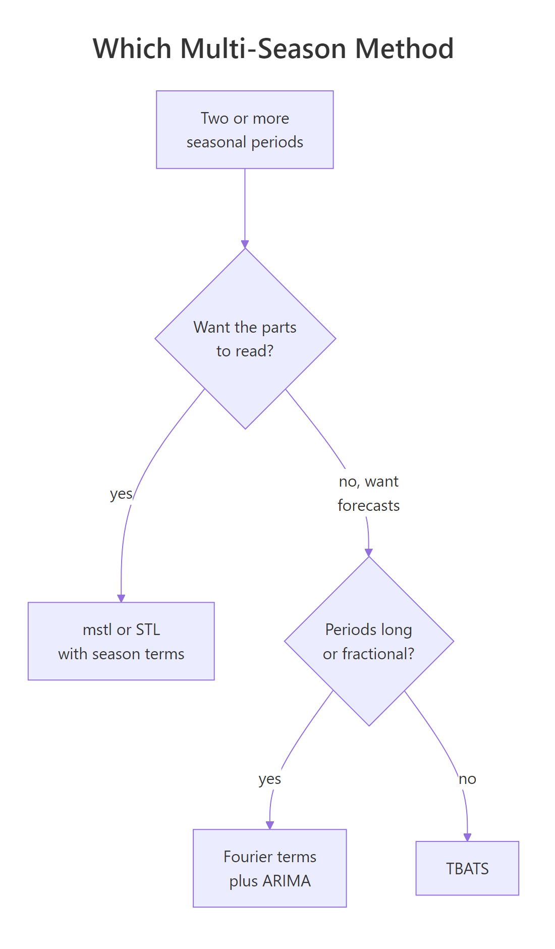
Figure 3: Choosing between MSTL, dynamic harmonic regression and TBATS for data with several seasonal periods.
Try it: The default forecast method for the seasonally adjusted series is ETS. Refit the one-day-ahead forecast with method = "naive" and see how much of the accuracy came from ETS.
Click to reveal solution
Explanation: Both score 132, because over a single day the seasonally adjusted series barely moves, so ETS and a flat naive line predict almost the same level. Almost all of the accuracy came from the seasonal components, not from the model fitted to what was left.
Complete Example: an end-to-end multi-season workflow
Here is the full routine on the simulated daily sales series from earlier, which has a weekly cycle and a yearly cycle. The workflow is the same four steps for any series: declare, decompose, check, then use.
Step one is to hold out the last 28 days and declare both periods on the training part.
Day one of the series sits 76 units below its yearly average because of where it falls in the year, and 28 units above because of the day of the week. Both effects are separated from a level of 503.
Step two is scoring the components so you know which ones matter.
Both are strong, with the yearly cycle dominating, which matches how the data was generated. Step three checks the remainder for structure the decomposition missed.
Neither lag 7 nor lag 14 shows a positive spike, so no weekly pattern survived into the remainder. Mildly negative values are what a smoother normally leaves behind when it removes a little genuine noise along with the pattern, and they are nothing to worry about.
Step four is putting the decomposition to work, and scoring it against the obvious benchmark.
The decomposition forecast misses by 14.5 units on average against 17.7 for seasonal naive, an 18 percent improvement. It wins here because seasonal naive only knows the weekly cycle, while MSTL also carries the yearly position and the drift forward.
Practice Exercises
Exercise 1: Does the weekend effect change over time?
Decompose only the most recent six weeks of taylor and compare the size of the weekly component with the full twelve-week decomposition. Use the standard deviation of Seasonal336 as the measure of size, and store the recent fit in my_fit.
Click to reveal solution
Explanation: The recent weekend effect is slightly smaller (2,623 against 2,733) but close, so the weekly pattern was stable across the summer. A big gap would have been a reason to use a smaller s.window so the shape could adapt.
Exercise 2: Write a reusable season report
Write a function season_report(x, periods) that decomposes any series at any set of periods and returns a data frame with one row per period, giving the seasonal strength and the peak-to-trough amplitude of that component. Test it on taylor with periods 48 and 336.
Click to reveal solution
Explanation: Building the column names from the periods with paste0() is what makes the function general. The report says the daily cycle moves demand by 14,174 megawatts from its lowest point to its highest, and the weekly cycle by 11,538.
Exercise 3: Catch a period you forgot to declare
Build an hourly series with a daily cycle and a weekly cycle, decompose it declaring only the daily period, and prove that the weekly cycle ended up in the trend. Use the standard deviation of the trend, and its correlation with the weekly component from a correct decomposition.
Click to reveal solution
Explanation: The series was built with no trend at all, yet the single-season decomposition reports a trend with a standard deviation of 10.09. That fake trend correlates 0.998 with the weekly component from the correct fit, which is as direct a proof as you can get that the undeclared cycle was absorbed by the trend.
Frequently Asked Questions
What is the difference between stl() and mstl()? stl() removes exactly one seasonal period, the frequency of the ts object. mstl() accepts a vector of periods and removes each one in turn using repeated stl() fits, and it also picks its own smoothing windows so you can call it with no arguments.
When should I use TBATS instead of MSTL? Use TBATS when forecasting accuracy matters more than interpretable components, and when the seasonal patterns are complex enough to need Fourier representation. MSTL is faster, and its output is far easier to explain to somebody who does not model time series for a living.
Can mstl() handle non-integer periods like 365.25? Yes. Declare seasonal.periods = c(7, 365.25) and you get a column named Seasonal365.25. You need at least two full cycles of data, so a yearly component on daily data needs roughly three years.
What happens to missing values? mstl() interpolates them with na.interp() before decomposing, then restores the NAs in the remainder afterwards. That is convenient, though a long gap will produce a confidently wrong interpolation, so check gaps before trusting the components around them.
Why do my components differ between forecast::mstl() and fable's STL()? Different default seasonal windows, and fable's STL() also lets you set robust = TRUE. Both are legitimate smoothers, and the components typically correlate above 0.9 on the dominant cycle while disagreeing more on the weaker one.
How do I decompose a multiplicative series? Pass lambda = "auto" so the series is Box-Cox transformed before decomposition, or take logs yourself first. Remember that the components then live on the transformed scale and no longer sum to the original data.
Is R's MSTL the same algorithm as the one in statsmodels? Both implement the same published method, from Bandara, Hyndman and Bergmeir. Default windows and iteration counts differ between the two libraries, so numbers will not match exactly even on identical data.
Summary
MSTL turns a series that repeats on several clocks into one readable component per clock, using nothing more exotic than repeated STL fits.
| What you want | How to do it |
|---|---|
| Declare several periods | msts(x, seasonal.periods = c(48, 336)) |
| Decompose | mstl(x) |
| Get components as columns | as.data.frame(fit) |
| Plot everything | autoplot(fit) |
| Let a shape drift or freeze it | s.window, numeric and odd, or "periodic" |
| Handle a multiplicative series | lambda = "auto" |
| Check for leftover cycles | remainder ACF at each seasonal lag |
| Rank the cycles | seasonal strength, or the component standard deviations |
| Forecast from it | forecast(fit, h = ...), then compare against snaive() |
| Do it in a tsibble | STL(y ~ season(period = 48) + season(period = 336)) |
The four-step routine that covers most work: declare the periods, decompose, check the remainder and the strengths, then use the seasonally adjusted series or the forecast. The single biggest mistake is declaring too few periods, because the missing cycle does not disappear, it is absorbed into the trend and the remainder instead.
References
- Hyndman, R. J. et al. - Multiple seasonal decomposition,
mstl()reference, forecast package. Link - Bandara, K., Hyndman, R. J. & Bergmeir, C. - MSTL: A Seasonal-Trend Decomposition Algorithm for Time Series with Multiple Seasonal Patterns. arXiv:2107.13462 (2021). Link
- Hyndman, R. J. & Athanasopoulos, G. - Forecasting: Principles and Practice (3rd ed), Section 12.1, Complex seasonality. Link
- Cleveland, R. B., Cleveland, W. S., McRae, J. E. & Terpenning, I. - STL: A Seasonal-Trend Decomposition Procedure Based on Loess. Journal of Official Statistics (1990). Link
- R Core Team -
stl()documentation, stats package. Link - O'Hara-Wild, M., Hyndman, R. J. & Wang, E. - STL decomposition reference, feasts package. Link
- Hyndman, R. J. - forecast: Forecasting Functions for Time Series and Linear Models, CRAN. Link
- O'Hara-Wild, M., Hyndman, R. J. & Wang, E. - vic_elec, half-hourly electricity demand for Victoria, tsibbledata. Link
Continue Learning
- Time Series Decomposition in R: STL vs Classical - the single-season foundation this tutorial extends, covering classical decomposition and plain STL.
- Time Series Features with feasts - turn seasonal strength and dozens of other measures into one row per series so you can triage hundreds at a time.
- Box-Cox and Transformations for Time Series in R - what the
lambdaargument is doing, and how to choose a transformation deliberately.