Cointegration in R: Engle-Granger and Error Correction
Two time series are cointegrated when each one wanders freely with no fixed level of its own, yet some fixed combination of the two does not wander: the gap between them keeps getting pulled back toward a stable value. That single distinction decides whether a regression between two trending series is a real long-run relationship or a statistical mirage. This post walks you from the mirage to a fitted error correction model, one runnable block at a time, using only base R plus two small packages, tseries and urca.
Why do two unrelated series look so strongly related?
Before any theory, here is the problem that makes cointegration necessary. I am about to create two number sequences using nothing but a random number generator. They are built independently. Neither one knows the other exists. Then I will regress one on the other, and the regression will look excellent.
Let's build them first.
What the code did: rnorm(250) drew 250 independent random numbers, and cumsum() turned them into a running total. So walk_a[2] is walk_a[1] plus a fresh random number, walk_a[3] is walk_a[2] plus another one, and so on. walk_b was built the exact same way from a completely separate draw.
A series built this way is called a random walk. The defining feature is that it has no home. A random walk does not have an average level that it returns to; wherever today's shock pushes it, that becomes the new starting point for tomorrow. Formally:
\[ y_t = y_{t-1} + \varepsilon_t \]
Here \(y_t\) is today's value, \(y_{t-1}\) is yesterday's, and \(\varepsilon_t\) is a fresh random shock with mean zero. Notice there is no term pulling \(y_t\) back to any particular number. Every shock is permanent, and they accumulate forever.
The opposite of this is a stationary series: one whose average level, spread, and general behaviour stay the same over time. A stationary series does have a home, and it keeps returning to it. A random walk is non-stationary.
Let's look at our two walks.
Both lines drift. Because both happen to drift in a broadly similar direction over this particular stretch, they look related. They are not. Now watch what ordinary regression says about them.
Read that output as you normally would. The slope on walk_a is 0.83 with a t-statistic of 40.53 and a p-value below \(2 \times 10^{-16}\). The R-squared is 0.8689, meaning walk_a supposedly explains 87 percent of the variation in walk_b. In a normal analysis you would write this up as a strong finding.
It is nonsense. We built the two series from separate random draws. There is no relationship to find. This is called a spurious regression, and Granger and Newbold documented it in 1974 [2].
The reason is worth understanding, because it explains everything else in this post. The t-statistic is computed as the coefficient divided by its standard error, and that standard error formula assumes the regression's leftover errors are stationary. Here they are not: subtract one random walk from a multiple of another random walk and you still have a random walk. The formula divides by a number that is far too small, so the t-statistic is inflated to a size that has nothing to do with evidence.
One dramatic example could just be bad luck. Let's find out how often this happens by repeating the whole experiment 500 times with fresh random walks each time.
The code generated 500 brand new pairs of unrelated random walks, ran a regression on each pair, and recorded whether the slope came out significant at the usual 5 percent threshold. If the t-test were working correctly, roughly 5 percent of these should be significant by chance. Instead 87.8 percent of them were.
That is the practical takeaway: when you regress one non-stationary series on another, a "significant" result is the default outcome, not evidence. Nearly nine times out of ten you will find a relationship that does not exist.
Try it: See whether the fake relationship survives a different seed. The block below regresses ex_b on fresh white noise, which is stationary, so the R-squared comes out near zero. Swap that noise for the random walk ex_a and watch what happens.
Click to reveal solution
Explanation: A different seed gives a different R-squared, 0.32 instead of 0.87, but the same verdict: a t-statistic of 10.8 and a p-value that rounds to zero, from two series with no connection whatsoever. The size of the fake effect varies; its presence does not.
What does it mean for two series to be cointegrated?
So regressing one wandering series on another is usually a trap. But sometimes two series genuinely do move together, and we need a way to tell that case apart. Cointegration is that test.
Here is the picture that makes it click, borrowed from Michael Murray's 1994 note in The American Statistician [9]. Imagine a woman walking home from a pub with her dog off the leash. Track the woman alone and her path is a random walk: she has no fixed position she returns to. Track the dog alone and the same is true. But the distance between them is not a random walk at all. Whenever the dog strays too far she calls it back, and whenever she strays the dog trots after her. The gap wobbles, but it always gets pulled back toward a small value.
That is cointegration. Each series is non-stationary on its own, but a particular combination of them is stationary.
Two pieces of standard vocabulary make this precise:
- A series is I(0), read "integrated of order zero", if it is already stationary. It has a home level and returns to it.
- A series is I(1), read "integrated of order one", if it is not stationary, but its period-to-period change is. Our random walks are I(1): the walk itself has no home, but the steps (
diff(walk_a)) are just the original random numbers, which certainly do.
Two I(1) series \(y_t\) and \(x_t\) are cointegrated if there is some number \(\beta\) such that
\[ z_t = y_t - \beta x_t \]
is I(0). The pair \((1, -\beta)\) is called the cointegrating vector, and \(z_t\) is the equilibrium gap: the amount by which the two series are currently out of line with their long-run relationship.
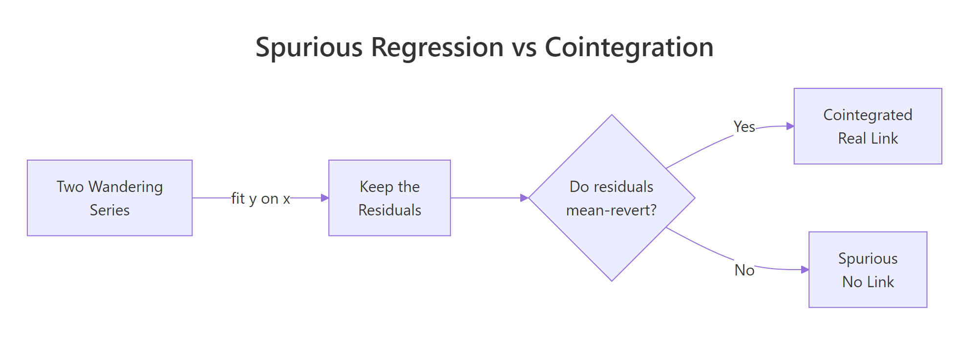
Figure 1: The single question that separates a real long-run relationship from a statistical mirage.
Now let's build a pair that really is cointegrated, so we have a known-good example to test against. A household's income and its spending make a natural story: spending tracks income over the long run, but in any given month a household can overspend or underspend, and that imbalance gets worked off over the following months.
Three lines did the real work. The income line makes a random walk with drift, so income wanders upward without ever settling at a level. The gap line makes a stationary AR(1) series, which means each month's gap is 75 percent of last month's plus a fresh shock, so it always decays back toward zero. The spending line combines them, which builds in the long-run rule "spending equals 20 plus 0.8 times income" and lets actual spending deviate from it temporarily.
Because we wrote the simulation, we know the true answers: the cointegrating slope is exactly 0.8, the intercept is exactly 20, and 0.75 of each month's gap carries over into the next, so a quarter of it disappears every month. Later we will check whether the statistics recover them.
Let's see what these two look like, and what their true gap looks like.
The top panel shows two series climbing from around 100 to around 138 with no fixed level. The bottom panel shows their gap hovering around zero the whole time, crossing the dashed line again and again. That contrast is the whole idea: the pieces wander, the combination does not.
Try it: Compute the true equilibrium gap using the coefficients we built into the simulation, then report its mean and standard deviation. The block below uses the wrong slope, 0.5, which leaves a trend behind and inflates the spread. Put the true 0.8 in and the gap collapses to something small and stationary.
Click to reveal solution
Explanation: The mean sits at -0.26 and the standard deviation is 0.90, so the gap stays within a couple of units of zero across all 240 months. Compare that to income, which travels nearly 40 units over the same period. The combination is anchored even though its ingredients are not.
How do you confirm both series are I(1) before testing?
Cointegration is only a meaningful question when both series are I(1). If a series is already stationary there is nothing to cointegrate, and the whole procedure would be answering a question nobody asked. So step zero is always a unit root test on each series separately.
The standard tool is the Augmented Dickey-Fuller test, adf.test() in the tseries package. Its null hypothesis is "this series has a unit root", which is another way of saying "this series is a random walk and therefore not stationary". A small p-value means you reject that, so a small p-value says stationary. A large p-value means you cannot reject it, so a large p-value says non-stationary.
That direction trips people up, so hold on to it: large p-value means non-stationary. For a full treatment of this test and its counterpart KPSS, see the stationarity testing post.
Let's run it on both of our levels.
Both p-values are enormous: 0.9618 for income and 0.8554 for spending. Neither one lets us reject the unit root, so we treat both as non-stationary. That is exactly what we want, because we built them that way.
Non-stationary is only half the definition of I(1). The other half is that the first difference must be stationary. diff() gives us the month-to-month change, and we test that too.
Both differenced series give p-values of 0.01, comfortably below 0.05, so we reject the unit root for each. Levels non-stationary, differences stationary: both series are I(1), and the cointegration question is now a legitimate one to ask.
Try it: We built gap to be stationary by construction. Confirm that the test agrees by running the ADF test on it directly.
Click to reveal solution
Explanation: A p-value of 0.0117 rejects the unit root, so gap is I(0), already stationary with no differencing needed. That is the property the whole Engle-Granger procedure is about to go looking for, except it will have to find it without knowing the true coefficients.
How does the Engle-Granger two-step test actually work?
The Engle-Granger procedure [1] turns the cointegration question into two things you already know how to do. Step one estimates the long-run relationship with ordinary least squares. Step two checks whether the leftovers from that regression are stationary.
The clever part is what the residuals mean. In step one we fit
\[ y_t = \mu + \beta x_t + u_t \]
and the fitted residual \(\hat{u}_t\) is our estimate of the equilibrium gap \(z_t\) from the previous section. So the residual is not a nuisance to be checked and forgotten. It is the exact quantity the theory cares about.

Figure 2: The Engle-Granger procedure end to end, from the I(1) pre-check to a fitted error correction model.
You might reasonably object at this point. Section one just showed that OLS between two I(1) series produces garbage, so why are we using OLS in step one? The answer is a genuinely surprising result called super-consistency. When the two series really are cointegrated, the OLS estimate of \(\beta\) converges on the truth faster than usual, at rate \(T\) rather than the usual \(\sqrt{T}\). The point estimate is trustworthy even though the standard errors and t-statistics printed beside it are not.
So we read the slope, and we ignore the stars.
The estimated slope is 0.785180 against a true value of 0.8, and the estimated intercept is 21.41 against a true value of 20. Super-consistency delivered: with 240 observations we have recovered the long-run relationship to within two percent, from data where the individual series never sit still.
The t-statistic of 132.68 beside that slope, on the other hand, tells us nothing. Section one produced a t-statistic of 40.53 from pure noise. Large t-statistics are what this kind of regression does.
Let's pull the residuals out and compare them against the residuals from the fake regression in section one.
The numbers hint at it and the plots make it obvious. The cointegrated residuals have a standard deviation of 0.889 and cross zero constantly, like a stationary series should. The spurious residuals have a standard deviation of 3.621 and stay far from zero for long stretches at a time, like a random walk.
Your eyes can tell these apart here. Step two of Engle-Granger is the formal version of that judgement, and the next section covers the one thing everybody gets wrong about it.
Try it: Confirm that the residuals really are the equilibrium gap by rebuilding them by hand from the fitted coefficients, then checking they match what residuals() returned.
Click to reveal solution
Explanation: The largest disagreement is about 0.000000000002, which is floating point rounding rather than a real difference. The residual is literally "how far spending is from where the long-run relationship says it should be", given this month's income.
Why are the printed critical values wrong for these residuals?
Step two asks whether ect has a unit root. It looks like the same job we did in section three, so the obvious move is to run a unit root test on it and read off the answer. That obvious move is the most common mistake in applied cointegration work, and this section is about why.
We will use ur.df() from the urca package rather than adf.test(), because it lets us control the specification. The regression it fits on the residual series is
\[ \Delta \hat{u}_t = \gamma \, \hat{u}_{t-1} + \sum_{i=1}^{k} \delta_i \, \Delta \hat{u}_{t-i} + \varepsilon_t \]
Where:
- \(\hat{u}_t\) is the residual from step one, our estimated equilibrium gap
- \(\Delta \hat{u}_t\) is this period's change in that gap
- \(\gamma\) is the coefficient of interest; \(\gamma = 0\) means a unit root, so the gap never closes
- \(\delta_i\) are lagged-change terms that mop up short-term autocorrelation
- \(\varepsilon_t\) is the leftover error
We set type = "none" because the residuals from a regression that already included an intercept have mean zero by construction, so adding another constant would be redundant. And lags = 1 sets \(k = 1\) in the formula above: one lagged-change term, which is enough for residuals this well behaved.
One R detail before the code. Objects from urca are S4 objects, and their parts come out with @ rather than the $ you would use on a list. So df_test@teststat is the test statistic and df_test@cval is the table of critical values that came with it.
The test statistic is -5.9985. R helpfully prints a table of critical values beside it: -2.58, -1.95 and -1.62 at the 1, 5 and 10 percent levels. Our statistic is far below all of them, so the naive reading is "reject the unit root, the residuals are stationary, the series are cointegrated".
The conclusion happens to be right. The critical values are wrong.
Here is why. Those numbers are Dickey-Fuller critical values, computed for testing a series you simply observed. Our residual series was not observed. It was manufactured by least squares, and least squares chooses \(\beta\) precisely to make those residuals as small as possible. OLS actively searches for the combination of the two series that looks most stationary. So even when no cointegrating relationship exists, the residuals it produces look more stationary than a randomly chosen combination would.
The null distribution of the test statistic therefore shifts to the left, and the correct thresholds are substantially stricter. The right table comes from MacKinnon [3], and depends on how many series are in the regression:
| Series in the regression | 1% | 5% | 10% |
|---|---|---|---|
| 2 (one regressor) | -3.90 | -3.34 | -3.05 |
| 3 (two regressors) | -4.29 | -3.74 | -3.45 |
| 4 (three regressors) | -4.64 | -4.10 | -3.81 |
For our two-series case the 5 percent threshold is -3.34, not -1.95. Our statistic of -5.9985 clears the stricter bar easily, so the verdict stands. But look what happens when we run the identical procedure on the fake pair from section one.
Read that carefully. The statistic is -1.9765. R's printed 5 percent critical value is -1.95, and -1.9765 is below -1.95, so anyone comparing against the printed table concludes that these residuals are stationary and declares the two series cointegrated.
They are two independent random walks. There is nothing there. Against the correct Engle-Granger threshold of -3.34, a statistic of -1.98 is nowhere close, and we correctly fail to reject.
The safer route is to let a purpose-built function handle it. ca.po() runs the Phillips-Ouliaris test [10], which is designed for exactly this job and prints critical values from the correct distribution. Its statistic works in the opposite direction from the ADF one: here a large value is the evidence for cointegration. Two arguments to know: demean = "constant" lets the two series sit at different fixed levels, the same job the intercept did in step one, and type = "Pu" picks the variance-ratio form of the statistic, which is the one the printed critical values belong to.
The genuinely cointegrated pair scores 106.97, which is more than triple the 5 percent threshold of 33.713. The spurious pair scores 17.122, below even the 10 percent threshold of 27.85. One clear yes, one clear no, and we did not have to look anything up.
Try it: The helper below hard-codes R's printed 5 percent value of -1.95, so it gives the spurious pair a clean bill of health. Change the threshold to the correct Engle-Granger value of -3.34 and watch the verdict flip.
Click to reveal solution
Explanation: The comparison is one-sided and points downward, because more negative means faster mean reversion. Swapping in -1.95 instead of -3.34 flips the second answer to "cointegrated", which is precisely the mistake this section exists to prevent.
How do you build an error correction model from the residuals?
Passing the test tells you a stable long-run relationship exists. It does not tell you anything about the short run: how quickly a household that overspent this month works the imbalance off, or how strongly next month's spending responds to next month's income. The error correction model, or ECM, answers both.
Granger's representation theorem says that any cointegrated pair can be written in error correction form. In plain words: if two series are tied together in the long run, then their short-run changes must contain a term that pulls them back whenever they drift apart. That pulling term is the lagged residual from step one.
The model is
\[ \Delta y_t = \mu + \gamma \, \Delta x_t + \alpha \, \hat{u}_{t-1} + \varepsilon_t \]
Where:
- \(\Delta y_t\) is this month's change in spending, the thing being predicted
- \(\Delta x_t\) is this month's change in income, and \(\gamma\) is the short-run response to it
- \(\hat{u}_{t-1}\) is last month's equilibrium gap, the error correction term
- \(\alpha\) is the speed of adjustment, the fraction of last month's gap closed this month
- \(\varepsilon_t\) is the leftover error
Everything in that equation is stationary, which means ordinary regression is valid again and the standard errors mean what they normally mean. That is the practical payoff of establishing cointegration first.
Building the pieces requires care with lengths, because differencing costs one observation.
The lag alignment is the part worth pausing on. diff(spending)[1] is the change from month 1 to month 2, so the gap that should explain it is the gap at month 1. Dropping the last element with ect[-n_obs] shifts the residual series back by exactly one period, so row i of the regression pairs month i's gap with the change from month i to month i+1. All three vectors now have 239 elements, which is what makes the regression run at all.
The regression predicted each month's change in spending from that month's change in income and the previous month's equilibrium gap. Three numbers carry the meaning.
The d_income coefficient is 0.85424. In the short run, a one unit rise in income this month raises spending by 0.85 units this month. Compare that to the long-run coefficient of 0.785 from step one: households respond a little more strongly on impact than the long-run relationship implies, and the difference gets unwound later.
The ect_lag coefficient is -0.24806, and this is the number the whole post has been building toward. It says that about 25 percent of last month's imbalance is corrected this month. If spending sat 4 units above where income says it should be, roughly 1 unit of that gets clawed back over the next month.
The sign matters enormously. Negative means correcting: being above the line pushes you down, being below pushes you up. And recall that we built the gap as an AR(1) with coefficient 0.75, which implies a true adjustment speed of \(0.75 - 1 = -0.25\). The estimate of -0.248 recovers it almost exactly.
A rate of 25 percent per month is easier to feel as a half-life: how long until half of a shock has been absorbed. If a fraction \(\alpha\) is corrected each period, the share still remaining after \(h\) periods is \((1 + \alpha)^h\), so setting that equal to one half and solving gives
\[ h = \frac{\ln(0.5)}{\ln(1 + \alpha)} \]
Half of any imbalance is gone within 2.43 months, and 81.9 percent of it is gone within six months. That is a fast-correcting relationship. The simulation's true half-life was \(\ln(0.5) / \ln(0.75) = 2.41\) months, so the estimate is accurate to within a week.
Half-life is what makes an adjustment speed interpretable across contexts. A pair of prices with a half-life of two days is an arbitrage relationship. A macroeconomic pair with a half-life of three years is a long-run tendency you would never trade on, even though both might show a statistically significant \(\alpha\).
Try it: The helper below computes a "90 percent life", the time until only 90 percent of a shock remains. Change the 0.9 to 0.5 to turn it into the half-life, then compare three different adjustment speeds.
Click to reveal solution
Explanation: Correcting 10 percent per period takes 6.58 periods to halve a shock, 25 percent takes 2.41, and 50 percent takes exactly 1 by definition. The relationship is strongly non-linear, so a slow-looking coefficient like -0.05 implies a half-life of over 13 periods.
When does Engle-Granger fail, and what do you use instead?
Everything so far worked because the example was cooperative. Engle-Granger has four real limitations, and knowing them is what separates using the method from trusting it blindly.
Limitation 1: the answer depends on which variable you put on the left. Regressing spending on income and regressing income on spending produce different residual series, so they produce different test statistics. There is no theoretical reason to prefer one.
The first line compares the slope we estimated directly, 0.7852, against the slope implied by inverting the reverse regression, 0.7958. The second line compares the two test statistics: -5.9985 and -5.8861. Both are far below -3.34, so the verdict is the same either way.
Now watch the same comparison on a shorter, noisier sample where the relationship is genuinely present but harder to see.
Same 90 observations, same true relationship, two opposite conclusions. Regressing short_y on short_x gives -1.981, which fails against -3.34 and says "not cointegrated". Regressing short_x on short_y gives -3.763, which passes comfortably and says "cointegrated". The second answer is the correct one, because we built the pair to be cointegrated with a stationary AR(0.93) gap.
The forward regression produced a false negative, and if you had only run it in that direction you would have thrown away a real relationship.
Limitation 2: with three or more series it can only ever find one relationship. Four series can share up to three independent cointegrating relationships. A single OLS regression returns a single residual series, so at best it finds one blend of them and reports it as if it were the whole story.
Limitation 3: the test has low power in short samples. The section above is an example. With 90 observations and a slowly correcting gap, the procedure often cannot tell a slow return from no return at all.
Limitation 4: a structural break will hide a real relationship. If the long-run coefficient changed partway through your sample, the residuals from a single fitted line contain a step, that step looks like a wandering component, and the test says no cointegration. Split the sample or use a break-aware test.
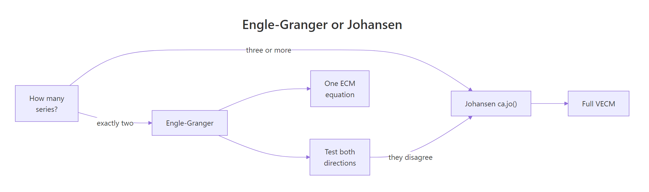
Figure 3: Choosing between Engle-Granger and Johansen.
The answer to limitations 1, 2 and 3 is the Johansen procedure [4], available as ca.jo() in urca. Instead of picking a left-hand-side variable and running one regression, it estimates a vector autoregression on all the series at once, which means every series is regressed on the recent past of every series including itself, and then asks how many independent cointegrating relationships the system contains. Because it treats every series symmetrically there is no direction to choose, and because it can find several relationships it scales past two series.
Its output is a sequence of trace statistics testing "at most \(r\) cointegrating relations" for \(r = 0, 1, 2, \dots\). You walk down the list and stop at the first row you cannot reject. Three arguments matter: type = "trace" asks for that sequence rather than the alternative maximum-eigenvalue version, ecdet = "const" allows a constant inside the long-run relationship (the counterpart of the intercept in step one), and K = 2 is the number of lags in the underlying vector autoregression, which is the smallest value the function accepts. Let's point it at the short sample that broke Engle-Granger.
The two statistics come out in the same order as the rows of the critical-value table printed under them, and that table runs from the largest \(r\) down to zero, so 6.17 belongs to r <= 1 and 21.37 belongs to r = 0. Read from the bottom row upward. The r = 0 row tests "there are no cointegrating relations": its statistic is 21.37 against a 5 percent critical value of 19.96, so we reject it and conclude there is at least one. The r <= 1 row tests "there is at most one": its statistic is 6.17 against 9.24, so we cannot reject it and we stop. Conclusion: exactly one cointegrating relationship.
Johansen found the relationship that the forward Engle-Granger regression missed entirely, on identical data. Let's also run it on the main simulated pair to see it recover the coefficients.
The trace statistic for r = 0 is 42.03, far above 19.96, and for r <= 1 it is 7.48, below 9.24. Exactly one relationship, same as before. The second output is the estimated cointegrating vector, normalised so spending has a coefficient of 1: it says spending minus 0.7745 times income minus 22.53 is stationary. The truth we simulated was spending minus 0.8 times income minus 20.
Try it: Run the Johansen test on the spurious pair from section one and check that it correctly finds nothing.
Click to reveal solution
Explanation: The r = 0 statistic of 16.40 sits below the 10 percent critical value of 17.85, so we cannot reject "no cointegrating relations". Johansen agrees with Phillips-Ouliaris and disagrees with the naive Dickey-Fuller table, which is a good summary of the whole post.
A Complete Example: Are the DAX and the SMI Cointegrated?
Everything so far ran on data we invented, where we knew the answer in advance. Now let's do the whole workflow on real market data and accept whatever it tells us.
EuStockMarkets ships with R. It holds 1,860 daily closing prices for four European stock indices from 1991 to 1998. We will take the German DAX and the Swiss SMI, two neighbouring markets that plausibly share a long-run relationship, and work in logs because price relationships are naturally proportional.
There are 1,860 trading days, and the log DAX climbs from 7.396 to 8.608 over the period, which is a rise of about 236 percent in price terms. A strongly trending series with no fixed level, exactly the setting where the spurious regression trap lives.
Step zero is the I(1) check on both series.
Both levels give p-values above 0.80, so neither is stationary. Both daily returns give 0.01, so both are stationary once differenced. Levels non-stationary, differences stationary: both series are I(1) and the question is legitimate.
Step one is the cointegrating regression.
This is the most convincing-looking regression output in the post. An R-squared of 0.965, a t-statistic of 226, three stars. Read by the usual rules it is a rock-solid relationship, and someone who skipped straight here would build a trading strategy on it.
But we have been trained. Section one produced a t-statistic of 40 from nothing at all, and the only thing that counts is whether the residuals are stationary. Step two.
Here is where the post's central lesson pays for itself. The residual statistic is -2.469. R's printed Dickey-Fuller 5 percent value is -1.95, so the naive comparison says "reject the unit root, these are cointegrated". Against the correct Engle-Granger 5 percent value of -3.34, the statistic falls well short and we cannot reject the unit root.
Phillips-Ouliaris agrees with the strict reading: 23.879 is below even the 10 percent critical value of 27.85. Two properly calibrated tests say the same thing. On this sample, the DAX and the SMI are not cointegrated, despite an R-squared of 0.965.
Let's fit the ECM anyway, because the adjustment speed shows what "not cointegrated" looks like in economic terms.
The short-run coefficient is strong and sensible: a 1 percent move in the SMI on a given day comes with a 0.78 percent move in the DAX the same day. These markets do trade together day to day.
The adjustment coefficient is -0.006384 with a p-value of 0.0107. It is negative, and with 1,859 observations it clears the 5 percent bar. But look at the size.
About 0.64 percent of a gap closes per day, which puts the half-life at 108 trading days, or roughly five months. Statistically detectable, economically irrelevant. A trader who spotted a 5 percent divergence would wait five months to capture half of it, and the residuals in the meantime range from -0.134 to +0.164, so the gap can easily double against them first.
For completeness, the second opinion from Johansen.
Johansen disagrees, mildly. Its r = 0 statistic of 24.43 exceeds the 5 percent value of 19.96, so it rejects "no cointegration" at the 5 percent level, though it falls just short of the 1 percent value of 24.60.
So we have a genuinely borderline case, and honesty is the right response. Engle-Granger and Phillips-Ouliaris say no; Johansen says a marginal yes; the estimated adjustment speed says any relationship is far too slow to act on. Report it as weak and inconclusive evidence, not as a finding. Real data does this often, and the discipline of naming the disagreement rather than quoting whichever test agreed with you is most of what good applied work consists of.
Frequently Asked Questions
What is the difference between correlation and cointegration? Correlation measures whether two series move together right now, and two independent random walks can be strongly correlated by accident, as section one showed. Cointegration is about the long run: it asks whether the gap between the series keeps getting pulled back to a stable value. Series can be highly correlated without being cointegrated, and cointegrated series can look weakly correlated over short windows.
Do both series have to be I(1)? Yes, for the standard procedure they must share the same order of integration. If one series is I(1) and the other is I(0), no linear combination of the two can be stationary except the trivial one, so the question is empty. If both are I(2) you can still test, but you need the I(2) machinery rather than the two-step method here.
Which variable should go on the left-hand side of the cointegrating regression? There is no statistical answer, which is exactly the weakness covered in section seven. Pick the one that makes economic sense as the dependent variable, then run the reverse regression as a robustness check. When the two directions give different verdicts, switch to ca.jo().
What if my adjustment coefficient comes out positive? Then the model is telling you deviations grow rather than shrink, which is not equilibrium behaviour. In practice this almost always means the residual test was a false positive or the specification is wrong. Go back to step two, check against the correct critical values, and do not report the model.
How many observations do I need? More than you think. The Engle-Granger test has low power in short samples, and section seven showed a genuinely cointegrated pair failing the test with 90 observations. Aim for at least 100, prefer several hundred, and treat a negative result from a short sample as inconclusive rather than as evidence of no relationship.
Can I use these tests on more than two series? ca.po() and lm() accept several regressors, but Engle-Granger will only ever find one relationship, and the correct critical value gets stricter as you add series, as the MacKinnon table in section five shows. For three or more series use ca.jo(), which is designed to count how many independent relationships exist.
Is cointegration the same as pairs trading? Pairs trading is one application of it. A trading strategy needs a stationary spread, which is what cointegration establishes, plus a half-life short enough that the trade closes inside your holding period. The DAX and SMI example shows why the second condition matters: a statistically significant adjustment speed with a half-life of five months is not a tradable signal.
Practice Exercises
These combine several parts of the workflow. Use fresh variable names so you do not overwrite anything from the tutorial.
Exercise 1: Test another pair of indices
Run the full Engle-Granger workflow on the French CAC and the British FTSE from EuStockMarkets, both in logs. Confirm both are I(1), fit the cointegrating regression, test the residuals with ur.df(), and give a verdict against the correct 5 percent critical value of -3.34.
Click to reveal solution
Explanation: Neither level rejects the unit root, so both are treated as I(1). The regression looks respectable with an R-squared of 0.7977, but the residual statistic of -1.0697 is nowhere near -3.34, and it does not even clear R's over-lenient -1.95. This is a clean negative: two trending indices, a decent-looking fit, and no cointegration at all.
Exercise 2: Write a reusable cointegration check
Write a function check_coint(y, x) that runs the whole two-step procedure and returns the estimated slope, the residual test statistic, and a verdict against -3.34. Apply it to three pairs: DAX and SMI, CAC and FTSE, DAX and CAC.
Click to reveal solution
Explanation: All three European index pairs fail, with statistics of -2.47, -1.07 and -2.03 against a threshold of -3.34. Every one of them would have been declared cointegrated by someone reading R's printed -1.95 for the first pair. Wrapping the correct threshold into a function is the cheapest possible defence against that mistake.
Exercise 3: Recover a known adjustment speed
Simulate a cointegrated pair whose gap is an AR(1) with coefficient 0.6, which means the true speed of adjustment is \(0.6 - 1 = -0.4\). Fit an error correction model and check how close the estimate lands, in both the coefficient and the half-life.
Click to reveal solution
Explanation: The estimated adjustment speed is -0.3885 against a true -0.4, and the estimated half-life is 1.409 periods against a true 1.357. The short-run coefficient of 1.2763 also lands close to the built-in long-run 1.3. With 300 observations and a fast-correcting gap, the procedure recovers everything it was designed to recover.
Summary
The whole workflow in one table.
| Step | What you are asking | R call | Decision rule |
|---|---|---|---|
| 0 | Is each series I(1)? | adf.test(x) and adf.test(diff(x)) |
Level p above 0.05 and difference p below 0.05 |
| 1 | What is the long-run relationship? | lm(y ~ x) |
Trust the slope, ignore the t-statistic |
| 2 | Is the equilibrium gap stationary? | ur.df(residuals(fit), type = "none", lags = 1) |
Compare to -3.34, not to R's printed -1.95 |
| 2b | Second opinion with correct values | ca.po(cbind(y, x), demean = "constant", type = "Pu") |
Large statistic is evidence for cointegration |
| 3 | How fast does the gap close? | lm(diff(y) ~ diff(x) + ect_lag) |
Adjustment coefficient must be negative and significant |
| 4 | Is that speed useful? | log(0.5) / log(1 + alpha) |
Read the half-life in your data's own time units |
| 5 | Three or more series, or a directional disagreement? | ca.jo(cbind(...), type = "trace", ecdet = "const", K = 2) |
Walk down the trace rows, stop at the first you cannot reject |
The points worth carrying away:
- Regressing one wandering series on another produces a significant result 87.8 percent of the time even when nothing is there. The t-statistic is not measuring evidence.
- Cointegration is the property that rescues the regression: the individual series wander, a fixed combination of them does not.
- The residual is the whole point of step one, not a diagnostic afterthought.
- R prints the wrong critical values for step two. Use -3.34 at 5 percent for two series, or let
ca.po()supply them. - The adjustment coefficient must be negative, and its half-life, not its p-value, tells you whether the relationship is worth using.
- Run both regression directions, and reach for
ca.jo()when they disagree or when you have more than two series.
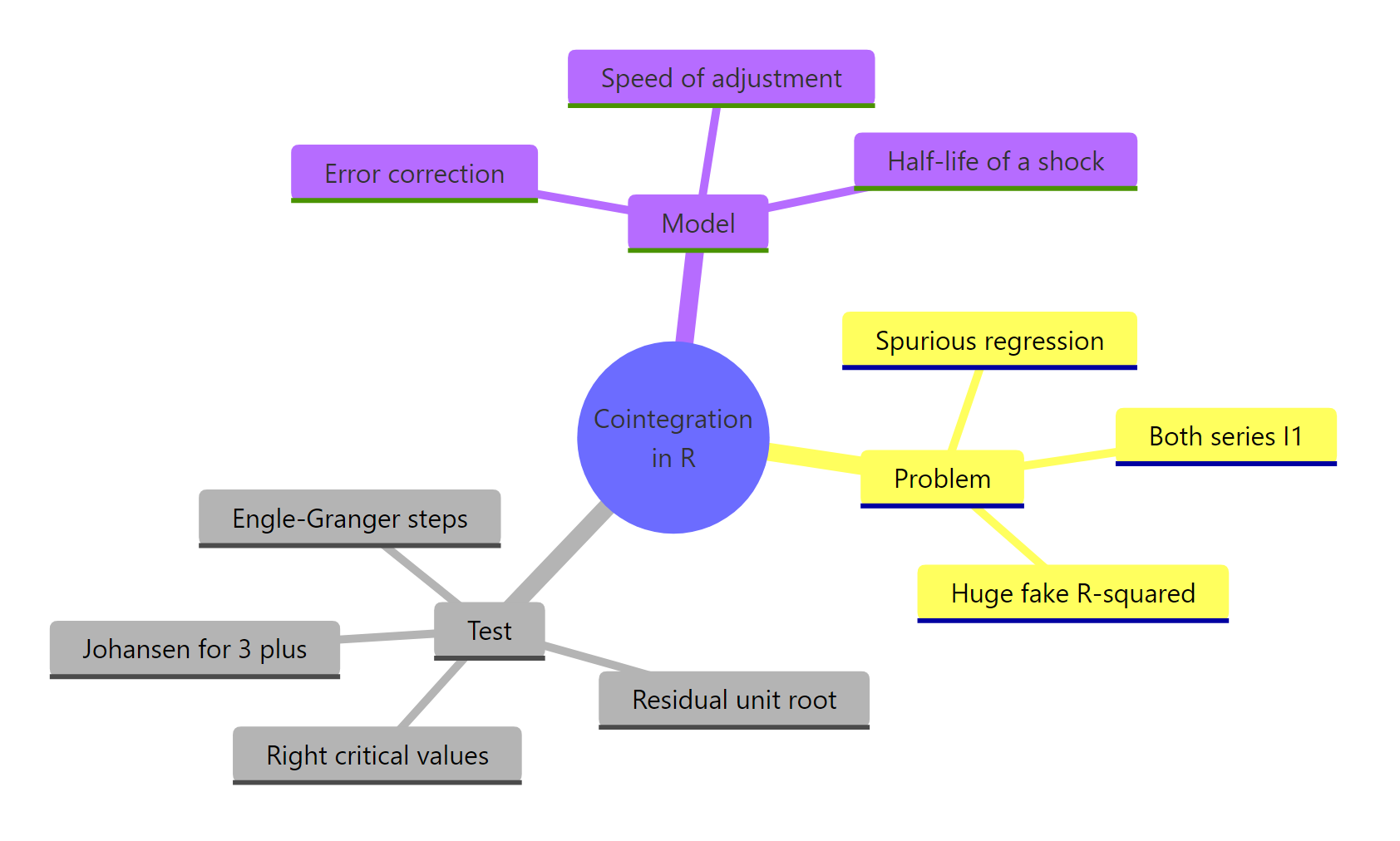
Figure 4: The whole workflow at a glance: the problem, the test, and the model.
References
- Engle, R. F. and Granger, C. W. J. Co-integration and Error Correction: Representation, Estimation, and Testing. Econometrica 55(2), 251-276 (1987). The paper that defines the two-step procedure and proves the representation theorem behind the ECM. Link
- Granger, C. W. J. and Newbold, P. Spurious Regressions in Econometrics. Journal of Econometrics 2(2), 111-120 (1974). The original simulation study of the trap in section one; short and very readable. Link
- MacKinnon, J. G. Critical Values for Cointegration Tests. Queen's Economics Department Working Paper No. 1227 (2010). Where the -3.34 comes from, with tables for more series and more specifications than this post covers. Link
- Johansen, S. Estimation and Hypothesis Testing of Cointegration Vectors in Gaussian Vector Autoregressive Models. Econometrica 59(6), 1551-1580 (1991). The source of the trace test, for readers who want the derivation behind
ca.jo(). Link - Pfaff, B. and Stigler, M. urca: Unit Root and Cointegration Tests for Time Series Data. CRAN reference manual. The argument-by-argument reference for
ur.df(),ca.po()andca.jo(). Link - Trapletti, A. and Hornik, K. tseries: Time Series Analysis and Computational Finance. CRAN reference manual. Documents exactly what
adf.test()fits and how it interpolates its p-values. Link - Pfaff, B. Analysis of Integrated and Cointegrated Time Series with R, 2nd Edition. Springer (2008). Book-length treatment by the author of
urca, including how to turn a Johansen result into a fitted vector error correction model. Link - Hyndman, R. J. and Athanasopoulos, G. Forecasting: Principles and Practice, 3rd Edition. OTexts. Free online text covering stationarity, differencing and unit roots in the wider forecasting context. Link
- Murray, M. P. A Drunk and Her Dog: An Illustration of Cointegration and Error Correction. The American Statistician 48(1), 37-39 (1994). The two-page note behind the walking analogy in section two, and still the clearest intuition available. Link
- Phillips, P. C. B. and Ouliaris, S. Asymptotic Properties of Residual Based Tests for Cointegration. Econometrica 58(1), 165-193 (1990). Explains why residual-based tests need their own null distribution, which is the point of section five. Link
Continue Learning
- Test Stationarity in R covers the ADF and KPSS tests in full detail, including how to read results that look contradictory and how to pick the number of differences.
- VAR Models in R is the natural next step after Johansen, since a vector error correction model is a VAR fitted to differenced series with the equilibrium gap added back in.
- ARIMA Models in R explains the differencing machinery that turns an I(1) series into a modellable one, which is the same operation the ECM performs on both sides.