How to Choose ARIMA Order (p,d,q) in R: ACF and PACF
Choosing an ARIMA order means fixing the three integers in ARIMA(p, d, q): d is how many times you difference the series to make it stationary, p (read from the PACF plot) is the number of autoregressive terms, and q (read from the ACF plot) is the number of moving-average terms. A residual white-noise check then confirms the order is good.
What does choosing an ARIMA order actually mean?
An ARIMA model is written ARIMA(p, d, q), and those three numbers are the only thing you have to decide. Everything else, the coefficients and the forecasts, R estimates for you once the order is set. So the whole job of "fitting an ARIMA model" really comes down to picking three small integers. This tutorial gives you a repeatable procedure for picking them instead of guessing.
The quickest way to see the goal is to let R pick an order automatically, then spend the rest of the tutorial learning to reproduce and judge that choice by hand. We will use the built-in Nile series, the annual flow of the river Nile from 1871 to 1970. This post assumes you already know what the AR, I, and MA pieces do; if not, read ARIMA in R first, then come back here for the order-selection recipe.
R settled on ARIMA(1,1,1). That is a fine answer, but a black-box answer. By the end of this tutorial you will be able to derive an order like it yourself, understand why each number was chosen, and know when to trust or override the automatic pick.
The whole process is four steps, always in the same order. Keep this table close; each section below is one row of it.
| Step | Question | Tool |
|---|---|---|
| 1. Find d | How many differences make it stationary? | ADF and KPSS tests, ndiffs() |
| 2. Find p | How many autoregressive terms? | the PACF plot |
| 3. Find q | How many moving-average terms? | the ACF plot |
| 4. Confirm | Is this order actually good? | AICc and a residual check |
The diagram below shows how those four steps flow into one another, including the loop back you take when the final check fails.
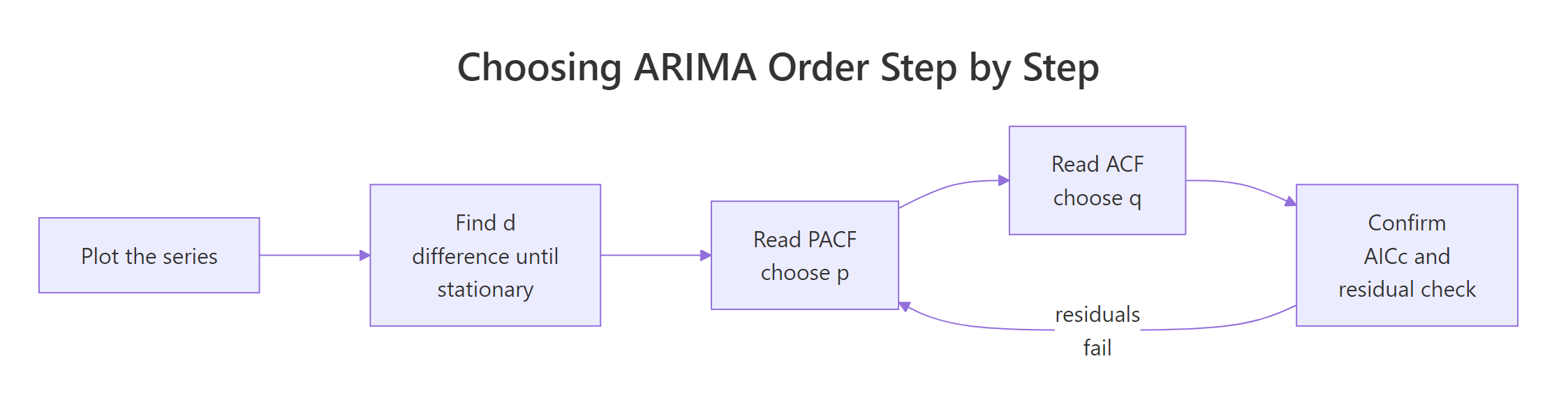
Figure 1: The four-step workflow for choosing an ARIMA order.
Before we start, here is a look at the raw numbers so you can picture the series behind that model.
The flow bounces around a high level early on, then tends to sit lower later in the record. That downward shift is a form of non-stationarity, and handling it is exactly what Step 1 is for.
Try it: Run an automatic fit on the LakeHuron series (annual lake levels) and read off its (p, d, q) from the label.
Click to reveal solution
Explanation: LakeHuron gets ARIMA(0,1,0), which reads as p = 0, d = 1, q = 0. That is a pure random walk: difference once, and no AR or MA terms are needed. Sometimes the right order really is that simple.
Step 1: how do you find d, the order of differencing?
The AR and MA parts of an ARIMA model both assume the series is stationary, meaning its average level and its amount of wobble stay roughly constant over time, with no trend drifting up or down. The Nile flow fails that test because its level shifts down partway through the record. The fix is differencing: instead of modeling the raw values, we model the change from one year to the next.
$$y'_t = y_t - y_{t-1}$$
Here $y_t$ is this year's value, $y_{t-1}$ is the previous year's value, and $y'_t$ is the difference between them, the change from one year to the next. The d in ARIMA(p, d, q) is just how many times you apply that operation. Most series need d = 0 or d = 1, and only rarely d = 2. Let us first look at the raw Nile flow to confirm the trend by eye.
The plot shows the level dropping around the year 1900, so the mean is not constant. Eyeballing is a start, but a formal test is more reliable. The Augmented Dickey-Fuller (ADF) test from the tseries package checks for a unit root, which is the mathematical signature of a series that needs differencing.
The ADF null hypothesis is that the series is non-stationary, and its alternative is stationary. The p-value of 0.0642 sits just above 0.05, so we cannot reject the null: the ADF test does not consider the raw Nile stationary. A second test, the KPSS test, comes at the question from the opposite direction, and running both together is good practice.
The KPSS null hypothesis is the reverse of ADF: it assumes the series IS stationary, so a small p-value is evidence AGAINST stationarity. Here the KPSS p-value is 0.01, which rejects stationarity. Both tests now agree the raw series needs differencing.
Rather than run and read the tests yourself, you can let the forecast package choose d for you. The ndiffs() function applies a stationarity test repeatedly and returns the number of differences required.
It returns 1, matching the d that auto.arima() chose at the top. Now let us confirm that a single difference actually does the job by re-running the ADF test on the differenced series. The diff() function turns levels into year-to-year changes.
The p-value drops to 0.01, so the differenced series clears the ADF test comfortably. We have our answer: d = 1, and we will do all further reading on nile_diff, the differenced series stored above.
ndiffs() says 1, resist the urge to difference again.Try it: Use ndiffs() to find how many differences the nhtemp series (yearly temperatures in New Haven) needs.
Click to reveal solution
Explanation: nhtemp needs one difference to remove its slow warming trend, so d = 1. Like most real series, a single difference is enough.
What do the ACF and PACF actually measure?
With the series made stationary, two plots do the rest of the work. They are the autocorrelation function (ACF) and the partial autocorrelation function (PACF), and together they are the heart of choosing p and q. If you want a slow, from-scratch treatment of these two plots, see the dedicated ACF and PACF guide; here we cover just enough to use them for order selection.
The ACF at lag k measures how correlated the series is with a copy of itself shifted k steps back. The PACF at lag k measures the same correlation but strips out the influence of all the shorter lags in between, so it captures only the direct link between a value and the one k steps earlier. That "direct link only" distinction is what makes the two plots tell you different things.
Both plots come with a shaded band, usually drawn as blue dashed lines. The band marks the range where a spike is small enough to be plausibly just noise. Its width is $\pm 1.96/\sqrt{n}$ for a series of length n, so a bar that pokes past the band is a "significant" spike worth paying attention to, while bars inside the band are treated as zero.
Two words describe how a plot behaves, and you need both:
- Cuts off: the bars are significant up to some lag, then drop abruptly inside the band and stay there.
- Tails off: the bars shrink gradually toward zero over many lags, often while alternating sign, without a clean break.
The ggtsdisplay() helper shows the series alongside both plots in a single view, which is the fastest way to inspect them. Let us look at the differenced Nile.
In that display, the ACF (bottom left) and PACF (bottom right) are what we will read in the next two steps. The sections that follow teach the exact rule for turning each plot into a number.
Try it: The Nile difference has 99 observations. Compute the width of the significance band for it.
Click to reveal solution
Explanation: The band sits at about plus or minus 0.197, so any ACF or PACF bar larger than roughly 0.2 in size counts as a significant spike for the differenced Nile.
Step 2: how do you read the PACF to choose p?
The rule for the autoregressive order is short: for a pure AR(p) process, the PACF cuts off sharply after lag p, while the ACF tails off gradually. So you find p by counting how many PACF spikes stick out past the band before it drops to near zero.
The cleanest way to trust that rule is to see it on data where we know the answer. Let us simulate a pure AR(2) series, whose PACF should show exactly two spikes and then nothing.
The plot shows two clear bars, then a drop inside the band. The numbers make it exact.
For 300 points the band is about plus or minus 0.113. R's PACF output starts at lag 1 (there is no lag-0 term, unlike the ACF you will see in Step 3), so these six values are lags 1 through 6. The first two (0.474 and -0.351), the PACF at lags 1 and 2, clear the band easily, and everything from lag 3 on sits inside. Two significant spikes, then a cutoff, is the textbook AR(2) fingerprint, so p = 2. That matches the two AR coefficients we used to build the series.
Now apply the same reading to the differenced Nile. Recall its PACF from the display above; here are the numbers.
Against a band of about plus or minus 0.2, the lag-1 bar (-0.402) is clearly significant, lag 2 (-0.246) is marginal, and the rest fade slowly rather than dropping off a cliff. There is no crisp cutoff here, which is the PACF tailing off. A tailing PACF points away from a large AR order, so p is small, most likely 0. We will let the ACF make the case for an MA term instead.
Try it: Simulate a pure AR(1) series and read its PACF. How many spikes stick out before it cuts off?
Click to reveal solution
Explanation: Only the lag-1 value (0.685) clears the band; everything after is inside it. One spike, then a cutoff, means p = 1, exactly the AR(1) we simulated.
Step 3: how do you read the ACF to choose q?
The rule for the moving-average order mirrors Step 2, with the two plots swapped: for a pure MA(q) process, the ACF cuts off sharply after lag q, while the PACF tails off gradually. So you count how many ACF spikes stick out before it drops inside the band.
Let us confirm on a simulated MA(1), whose ACF should spike once and then cut off.
The plot shows a single tall bar at lag 1, then a drop into the band. Here are the numbers.
The first value is always 1.000, the correlation of the series with itself at lag 0, so ignore it. The lag-1 value (0.502) is a clear spike, and from lag 2 on the bars sit at or inside the plus or minus 0.113 band. One significant spike, then a cutoff, is the MA(1) fingerprint, so q = 1.
Now read the ACF of the differenced Nile.
Ignoring the lag-0 value of 1.000, only the lag-1 bar (-0.402) clears the band of about plus or minus 0.2; every later bar is well inside it. That is a clean cutoff after lag 1, the signature of an MA(1). Put together with the tailing PACF from Step 2, the differenced Nile reads as MA(1), which means a candidate order of ARIMA(0, 1, 1): zero AR terms, one difference, one MA term.
The table below is the full reading rule. It is worth memorizing, because it covers every case you will meet.
| ACF behavior | PACF behavior | Suggested model |
|---|---|---|
| Tails off gradually | Cuts off after lag p | AR(p) |
| Cuts off after lag q | Tails off gradually | MA(q) |
| Tails off gradually | Tails off gradually | Mixed ARMA (compare by AICc) |
The diagram below turns that table into a decision you can follow at a glance.
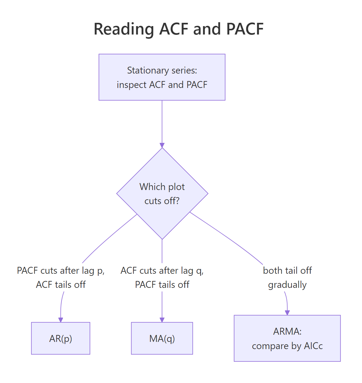
Figure 2: How the ACF and PACF point to an AR, MA, or mixed ARMA model.
Try it: Simulate a pure MA(2) series and read its ACF. How many spikes clear the band?
Click to reveal solution
Explanation: Ignoring the lag-0 value, the lag-1 (0.622) and lag-2 (0.268) bars both clear the band, and everything after is inside it. Two significant spikes, then a cutoff, means q = 2.
Step 4: how do you confirm the order with AICc and residual checks?
Reading the plots gave us a candidate, ARIMA(0, 1, 1), but a candidate is not a verdict. Step 4 tests it two ways. First, compare a shortlist of nearby orders by their AICc, a score that rewards good fit and penalizes needless complexity, where lower is better. Let us line up the ACF-suggested model against a few neighbors.
The lowest score belongs to ARIMA(1,1,1) at 1267.51, the same model auto.arima() picked. Our hand-read ARIMA(0,1,1) comes in at 1269.22, higher by only 1.71. A widely used rule of thumb says that when two models are within about 2 AICc points, they are essentially indistinguishable, so the tie-breaker is simplicity. The ARIMA(0,1,1) uses one coefficient instead of two, so the parsimonious choice is to keep the model our ACF identified.
The second test is the decisive one. A good model leaves behind residuals, the leftover one-step errors, that look like pure random noise. If a pattern remains, the model missed something. The checkresiduals() function runs a Ljung-Box test and draws the diagnostic plots in one call.
The Ljung-Box null hypothesis is that the residuals are just noise, so here we WANT a large p-value. At 0.1458 we cannot find leftover structure, which means the residuals pass as white noise and the order is confirmed. The plots it draws, a residual series with its own ACF and a histogram, should show no obvious pattern to back that up.
Try it: Fit the ARIMA(1,1,1) that auto.arima() preferred and read its AICc. How far below the 1269.22 of ARIMA(0,1,1) does it really sit?
Click to reveal solution
Explanation: The rival scores 1267.51 against 1269.22, a gap of 1.71. That is inside the 2-point rule of thumb, so the two models are practically tied and the simpler ARIMA(0,1,1) is the better everyday choice.
Complete Example: choosing an order for BJsales end to end
Let us run the full four-step procedure once more on a fresh series, this time landing on a different shape of model. The built-in BJsales series is a sales record from Box and Jenkins themselves, the statisticians who created this whole method. First, plot it.
The series climbs steadily, a clear trend, so Step 1 will call for differencing. Let ndiffs() decide.
One difference. Now inspect the differenced series with the combined display, then read the two plots.
The band here is about plus or minus 0.16. The PACF has two bars above it (0.312 and 0.200) and then drops inside, which looks like a cutoff after lag 2. The ACF, ignoring lag 0, stays positive and fades slowly, which is a tail. A PACF cutoff with a tailing ACF points to AR(2), so our shortlist starts with ARIMA(2, 1, 0). Let us compare it against a few neighbors by AICc.
Here the numbers overrule the eyeball read. The AR(2) we shortlisted scores 520.09, but the mixed ARIMA(1,1,1) scores 514.90, better by more than 5 points, well past the 2-point rule. When a plot suggests one thing and AICc strongly prefers another, follow the data: revise the choice to ARIMA(1, 1, 1). Confirm it with a residual check.
The Ljung-Box p-value of 0.6605 is comfortably large, so the residuals are white noise and ARIMA(1, 1, 1) is confirmed. With the order settled, forecasting is one call.
The point forecasts drift gently upward, continuing the trend, and the intervals widen further out as uncertainty compounds. This example carries the most important lesson of the whole tutorial: the ACF and PACF give you a smart starting shortlist, but AICc and the residual check make the final call.
Frequently Asked Questions
Do I read the ACF for p or for q? The ACF gives you q, the moving-average order, because an MA(q) process has an ACF that cuts off after lag q. The PACF gives you p, the autoregressive order. An easy way to remember it: the Partial ACF pairs with the p term.
How do I know when an ACF or PACF spike is significant? Compare it to the shaded band, which sits at plus or minus $1.96/\sqrt{n}$. A bar that pokes past the band is significant; a bar inside the band is treated as zero. For 100 observations the band is about plus or minus 0.2.
What if both the ACF and PACF tail off gradually? That is the signature of a mixed ARMA process, where neither plot gives a clean cutoff. In that case the plots cannot pin down the order alone, so fit a small grid of candidates and pick by AICc, which is exactly what auto.arima() automates.
Should I read the plots on the raw series or the differenced one? Always on the differenced, stationary series. The AR and MA parts only make sense once the trend is removed, so reading the ACF and PACF of a trending raw series will mislead you.
If auto.arima() picks the order for me, why learn to read the plots? Because auto.arima() can be wrong, and you need to judge it. Reading the plots and residuals lets you sanity-check its answer, override it when domain knowledge or a residual failure demands, and understand what the model is actually doing.
Can I over-difference a series? Yes, and it hurts. Differencing more than needed injects artificial negative autocorrelation at lag 1 and inflates the variance, which corrupts the ACF and PACF. Trust ndiffs() and stop as soon as the series is stationary.
Practice Exercises
These combine the four steps into fuller challenges. Each starter block runs as-is so you can experiment; write your own solution, then reveal ours to compare. The exercises use their own variable names so they will not clash with the code above.
Exercise 1: Identify the order for lh
The lh series records luteinizing hormone levels in blood samples. Work through all four steps: find d with ndiffs(), read the ACF and PACF, then compare a shortlist by AICc. What does a thorough auto.arima() settle on, and does it match your read?
Click to reveal solution
Explanation: The tests give d = 0, so no differencing. The plots are ambiguous: both the PACF and ACF have a strong lag-1 spike and then borderline values, so the eye cannot cleanly separate AR from MA. This is the "both tail off" case, so AICc breaks the tie. Among the candidates, ARIMA(0,0,2) scores lowest at 63.99, and the thorough auto.arima() agrees, landing on a pure MA(2).
Exercise 2: Identify a mystery series
Run the setup below to build a series without peeking at how it was made, then use the full workflow to recover its (p, d, q). Confirm your answer with a residual check.
Click to reveal solution
Explanation: ndiffs() gives d = 0. The PACF has two significant spikes (0.453 and -0.357) then cuts off, while the ACF tails off, the classic AR(2) fingerprint, so the read is ARIMA(2, 0, 0). AICc confirms it (962.65 beats both neighbors), and the Ljung-Box p-value of 0.5216 says the residuals are white noise. The order is ARIMA(2, 0, 0), which is exactly the process the setup simulated.
Exercise 3: When d itself is in doubt
LakeHuron is a famous puzzle. Its ndiffs() says difference once, yet the PACF of the raw levels shows a clean AR(2) shape. Read the PACF of the levels, note what ndiffs() says, then fit ARIMA(2,0,0) on the levels and check its residuals. Why can you NOT settle this by comparing the AICc of the two models?
Click to reveal solution
Explanation: The PACF of the levels cuts off after lag 2 (0.832 and -0.267 are significant), pointing to AR(2) with no differencing, while ndiffs() leans toward one difference. Both are defensible: this is the trend-stationary versus difference-stationary judgment call. You cannot decide it by AICc, because ARIMA(2,0,0) is fit to the levels and a differenced model is fit to the changes, so their AICc values are on different scales. Instead you judge by residual diagnostics and context. Here the AR(2) on the levels passes cleanly (Ljung-Box p = 0.6533), which is why it is the textbook model for this series.
Summary
Choosing an ARIMA order is a four-step routine you can run on any series: find how much differencing makes it stationary, read the PACF for the AR order, read the ACF for the MA order, then confirm with AICc and a residual check. The plots nominate; the diagnostics decide.
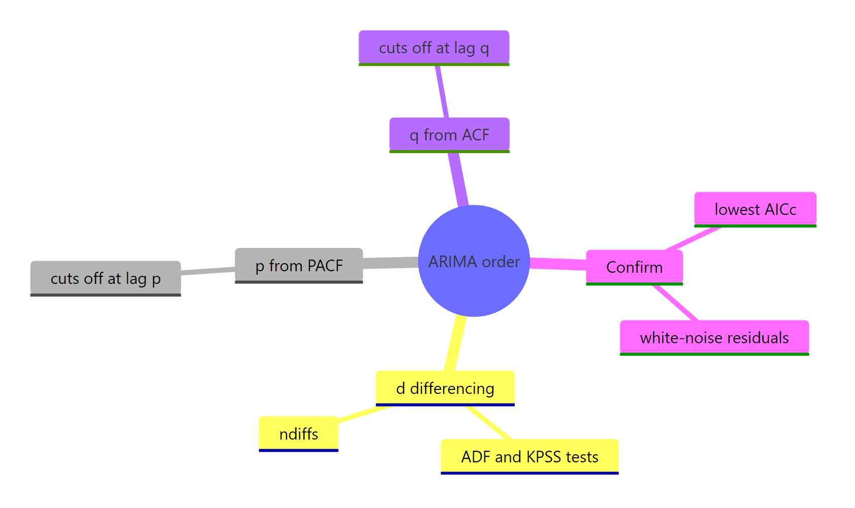
Figure 3: Overview of the whole order-selection process, from differencing to confirmation.
| Step | What you decide | Key function | Reading rule |
|---|---|---|---|
| Find d | Order of differencing | ndiffs(), adf.test(), kpss.test() |
Difference until stationary |
| Find p | AR order | Pacf() |
PACF cuts off after lag p |
| Find q | MA order | Acf() |
ACF cuts off after lag q |
| Confirm | Whether the order is good | Arima(), checkresiduals() |
Lowest AICc plus white-noise residuals |
Keep these takeaways close:
- The PACF gives p, the ACF gives q. A sharp cutoff after lag k in the PACF means p = k; a sharp cutoff in the ACF means q = k. When both tail off, it is a mixed model and AICc decides.
- Always read the plots on the stationary, differenced series. Decide d first with
ndiffs(), and only compare AICc between models that share that d. - A significant spike pokes past the plus or minus $1.96/\sqrt{n}$ band. Bars inside the band are noise.
- The residual check is the final word. No order is confirmed until
checkresiduals()shows white noise, and a small AICc gap between two passing models breaks in favor of the simpler one.
References
- Hyndman, R.J., & Athanasopoulos, G. - Forecasting: Principles and Practice, 3rd edition. Chapter 9.5: Non-seasonal ARIMA models and order selection. Link
- Hyndman, R.J., & Khandakar, Y. - "Automatic Time Series Forecasting: The forecast Package for R." Journal of Statistical Software, 27(3), 2008. Link
- Box, G.E.P., Jenkins, G.M., Reinsel, G.C., & Ljung, G.M. - Time Series Analysis: Forecasting and Control, 5th edition. Wiley (2015). Chapter 6: Model identification.
- forecast package -
ndiffs()reference. Link - forecast package -
Arima()reference. Link - R Core Team -
acf()andpacf()documentation, An Introduction to R. Link
Continue Learning
- ARIMA in R - the companion guide on what AR, I, and MA mean and how to fit and forecast an ARIMA model.
- ACF and PACF in R - a from-scratch look at the two plots at the center of this workflow.
- Test Stationarity in R - the full set of unit-root and stationarity tests behind the differencing step.