Time Series Objects in R: ts, xts, zoo, or tsibble?
R does not have one time series type, it has four: ts from base R, plus zoo, xts and tsibble from packages. They differ in one important way: where they keep the "when" that belongs to each number. ts computes the dates from a start and a frequency, so it only works on a perfectly regular grid; zoo and xts store a real index of dates beside the values, so gaps and irregular timestamps survive; tsibble puts the index in a column of a tidy table and adds a key so many series fit in one object. This post builds all four from the same data, shows the exact point where ts silently gets the dates wrong, and ends with a rule for choosing.
Everything below uses one small business, so you always have something concrete to picture.
Riverside Roasters is a coffee shop. We will use two of its datasets:
- Monthly revenue, January 2023 to December 2025. That is 36 numbers, one per month, none missing. A perfectly regular grid.
- Daily cups sold, Monday 3 March to Saturday 15 March 2025. That is 12 numbers, because the shop is closed on Sundays. Sunday 9 March simply does not exist in the data.
That single closed Sunday is the most useful thing in this post. It is the thing that breaks ts, the thing zoo and xts handle without complaint, and the thing tsibble insists on naming out loud.
What is a time series object, and why not just use a vector?
A time series is two things glued together: the values (what happened) and the index (when it happened). The index is the list of time points, one per value. A plain R vector holds only the values. The "when" has to live somewhere else, in your head or in a separate column, and anything you keep separately can drift apart from the data it describes.
A time series object glues the index to the values so the two can never separate. Here is Riverside's monthly revenue, first as a bare vector of numbers, then as a ts object. Watch what ts() gives you for free.
Read the call first. revenue is an ordinary vector of 36 numbers built from a rising trend (500 * (1:36)) plus random noise; set.seed(42) just makes the random numbers the same every time you run it, so your screen matches the numbers here. Then ts(revenue, start = c(2023, 1), frequency = 12) wraps that vector. start = c(2023, 1) means the first value belongs to the 1st period of 2023. frequency = 12 means there are 12 periods in a year, so a period is a month.
Now look at what printed. We never handed R a single date, yet it laid the numbers out in a calendar: years down the side, months across the top, revenue climbing from 19,734 in January 2023 to 34,455 in December 2025. That is the payoff of a time series object. From start and frequency alone, ts worked out that the 15th number belongs to March 2024 and printed it there.
That labelling is not decoration. Because the index is attached, you can ask for data by calendar time instead of by position:
Both lines return the same number, 25380, and that is exactly the point. To get it from the vector you had to know that March 2024 is the 15th month, which means you did the calendar arithmetic in your head. window() did it for you, and it printed Mar 2024 next to the answer as proof. window(x, start, end) pulls out the slice of a time series between two time points, inclusive.
Scale that up. When you have 4,000 rows of sensor readings and you want "the week of the outage", counting positions by hand stops being a small annoyance and starts being a source of quiet, unnoticed mistakes.
How does ts store time, and where does it break?
Here is the one detail about ts that everything else in this post follows from: a ts object does not store your dates. It stores two numbers and computes the dates on demand.
Take rev_ts apart and you can see it. There are only a handful of pieces:
Walk through each one. start() gives the first time point as c(year, period), so period 1 of 2023. end() gives the last, period 12 of 2025. frequency() is the number of periods per unit of time, 12 here. deltat() is the gap between two neighbouring observations, expressed as a fraction of a year: 1/12 = 0.08333333.
time() is the interesting one. It returns the index, and the index is a plain number line: January 2023 is 2023.000, February is 2023.083, March is 2023.167. Each step adds exactly 1/12. Those are not dates. They are evenly spaced decimals, computed by the formula
$$t_i = \text{start} + \frac{i - 1}{f}$$
where \(t_i\) is the time of the \(i\)-th observation, \(\text{start}\) is the starting time as a decimal (2023.0), \(i\) is the position (1, 2, 3, ...) and \(f\) is the frequency (12). Check the third value with your own arithmetic: \(2023 + (3-1)/12 = 2023.1\overline{6}\), which is the 2023.167 that printed for March.
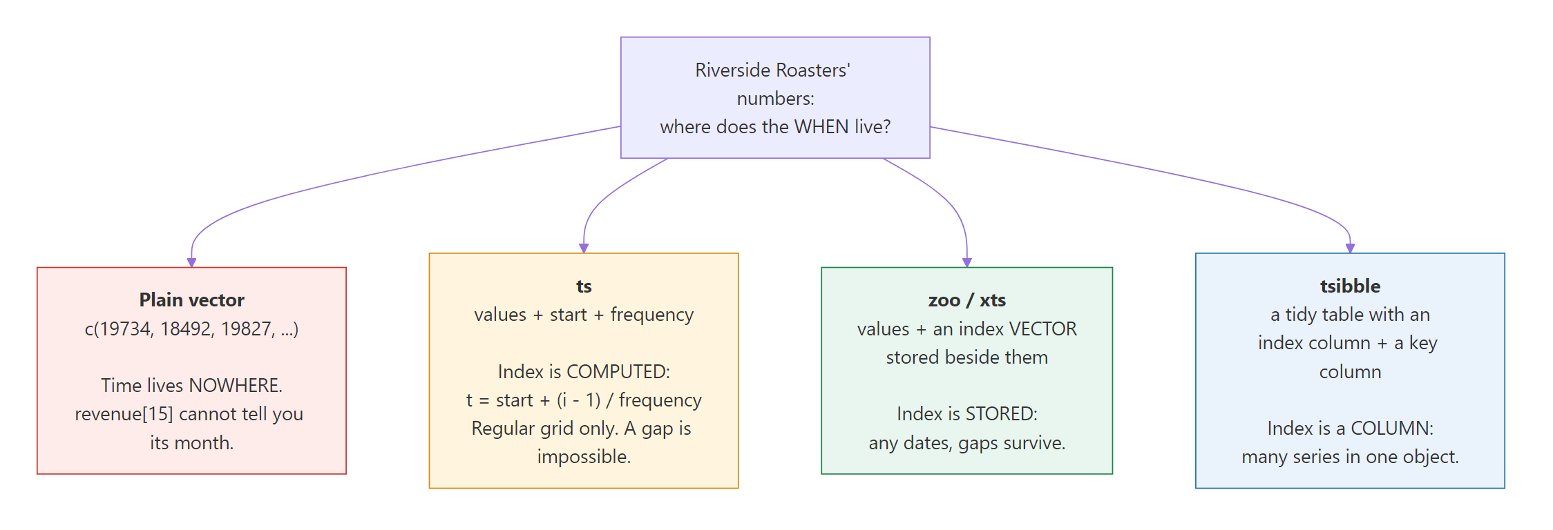
Figure 1: The one thing that separates the four classes. A ts computes its index from start and frequency, so every observation must sit on an evenly spaced grid. zoo and xts store the index, so it can be anything.
Now stare at that formula and ask the question this whole post turns on: where in \(t_i = \text{start} + (i-1)/f\) could you put a gap?
There is nowhere. The formula marches forward in equal steps of 1/f forever. The \(i\)-th observation is defined to be one step after the \((i-1)\)-th. A ts object cannot represent a missing Sunday, because "the next observation" and "one step later" are the same statement.
So what happens if you hand ts() gapped data anyway? It does not warn you. It counts.
There is a lot in that block, so take it in pieces. seq(as.Date(...), as.Date(...), by = "day") builds every calendar day from 3 to 16 March. format(all_days, "%u") returns the weekday as a number where Monday is 1 and Sunday is 7, so keeping the days where it is not "7" drops the two Sundays and leaves the 12 days the shop was open. ts(cups, start = c(2025, 62), frequency = 365) then declares "365 periods per year, starting at day 62", and day 62 of 2025 really is 3 March.
The last three lines just run the index formula backwards to ask bad_ts what date it believes each observation has, so we can print its belief next to the truth.
Now read the table, and read it row by row. Observations 1 through 6 are correct: 3 March through 8 March, Monday to Saturday. Then look at row 7. The truth is Monday 10 March, because the shop was shut on the 9th. But ts says 9 March. It had no way to know a day was skipped, so it did the only thing the formula allows: it added one step and moved on.
And it never recovers. Every observation from row 7 to row 12 is stamped one day early, so the last one is filed under Friday 14 March when it was really Saturday the 15th.
Watch out: No error was raised. No warning.
bad_tsprints, plots and models perfectly happily, and every date in it from the 7th observation onward is wrong. This is one of the most expensive mistakes you can make in R time series work, because the code looks fine and the numbers look fine. If you then fit a weekly seasonal model, it is learning a seasonality that your data does not have.
The lesson is not "ts is bad". ts is excellent, and for the monthly revenue it is the best tool in this post. The lesson is that ts assumes a regular grid and cannot check that assumption for you. When the assumption holds, its computed index is a feature. When it does not, you need a class that stores the dates instead of computing them.
What does zoo do differently?
zoo (Z's Ordered Observations, after its author Achim Zeileis) changes exactly one thing, and everything else follows from it: it stores the index as a real vector sitting beside the values. Nothing is computed, so nothing has to be evenly spaced.
You build one with zoo(values, order.by = index), where order.by is the actual "when" of each value.
The printed object already shows the difference: real dates above the numbers, not a computed grid. The two accessor functions split the object into its halves. index() returns the "when" (a vector of Date values) and coredata() returns the "what" (the plain numeric vector). Those two names are worth memorising, because they work on zoo and xts objects alike and they are how you get your data back out.
Because the dates are stored rather than inferred, asking for a range gives an honest answer:
We asked for five calendar days and got four numbers back: the 7th, 8th, 10th and 11th. Sunday the 9th is not there, was never there, and zoo did not quietly promote the 10th into its place the way bad_ts did. Compare that output to row 7 of the earlier table and you have the whole argument for storing an index in one line.
Sometimes you want the opposite: to make the hole visible rather than skip over it. Merge the data against a zoo that holds every calendar day and the missing days show up as NA:
zoo(, all_days) looks like a typo but is not: leaving the values argument empty creates an empty zoo that carries an index and no data. Merging our cups against it lines both indexes up and fills the unmatched slots with NA. Both Sundays, the 9th and the 16th, now appear as explicit NA holes. That is often what you want before plotting, because a chart of cups_full draws a break at each closed Sunday instead of a straight line pretending the shop was open.
zoo also brings the rolling and aggregating tools that make this class worth loading:
rollmean(x, k = 3) slides a 3-wide window along the series and averages each window. The first value, 323.3333, is the mean of the first three cups counts (377, 290 and 303), and it is labelled 4 March because that is the middle of that window. Note carefully what "3" counts here: three observations, not three calendar days. Over the Sunday boundary a window spans Saturday, Monday and Tuesday. That is usually the sensible reading for a shop that closes on Sundays, but it is a decision you are making, so make it knowingly.
When should you use xts instead?
xts (eXtensible Time Series) is built directly on top of zoo. It keeps the stored index and adds two things: the index is guaranteed to be a real date or time class (never an arbitrary label), and you get a much sharper set of tools for slicing by calendar, which is why it became the standard in finance.
One note before the code. The xts and tsibble blocks in this post are marked "run locally" because those two packages are not available in the in-browser R session that runs the live blocks above. Everything else on this page runs in your browser as-is. Install these two once with install.packages(c("xts", "tsibble")) and every block below works exactly as printed.
The headline feature is subsetting with a date string:
library(xts)
cups_xts <- xts(cups, order.by = open_days)
colnames(cups_xts) <- "cups"

cups_xts["2025-03-10/2025-03-12"]
#>            cups
#> 2025-03-10  339
#> 2025-03-11  317
#> 2025-03-12  324
periodicity(cups_xts)
#> Daily periodicity from 2025-03-03 to 2025-03-15
The string "2025-03-10/2025-03-12" is an ISO-8601 date range: everything from the 10th to the 12th. No window(), no as.Date() wrapping, no positions. periodicity() inspects the index and reports what the spacing actually is, which is a quick sanity check when you inherit data and do not yet trust its shape.
The string subsetting gets more useful the coarser you go. Give it only a month and it hands you the whole month:
cups_xts["2025-03"]
#>            cups
#> 2025-03-03  377
#> 2025-03-04  290
#> 2025-03-05  303
#> 2025-03-06  310
#> 2025-03-07  296
#> 2025-03-08  296
#> 2025-03-10  339
#> 2025-03-11  317
#> 2025-03-12  324
#> 2025-03-13  375
#> 2025-03-14  329
#> 2025-03-15  388
endpoints(cups_xts, on = "weeks")
#> [1]  0  6 12
cups_xts["2025-03"] returned all of March, and notice it returned 12 rows, not 14: the closed Sundays are still absent, exactly as they should be. "2025" would give you the whole year, and "2025-03-10/" would mean "the 10th onward".
endpoints(x, on = "weeks") reports the row positions where each week ends: 0, 6 and 12. Read it as boundaries rather than data, always starting at 0. Rows 1 to 6 are the first week (Monday the 3rd to Saturday the 8th) and rows 7 to 12 are the second. That is what you feed to period.apply() to aggregate by week, and it is why "give me weekly totals from daily data" is a one-liner in xts rather than a date-arithmetic puzzle.
Use xts when your data has real timestamps and you slice by calendar a lot: stock prices, sensor logs, anything intraday. Use zoo when you want the same stored-index idea but with an index that is not a date at all, since zoo will happily order by any sortable vector.
What makes tsibble different?
The three classes so far share a limitation that is easy to miss: none of them can label which series a value belongs to. rev_ts is Riverside's revenue. cups_zoo is Riverside's cups. The moment Riverside opens a second location, you have two series, and your options with ts or xts are to juggle two separate objects or to bolt the two series together as extra columns, which forces both shops onto one shared index whether or not that is true of the data.
tsibble takes a different route. It is a tidy data frame (so dplyr verbs work on it) that knows which column is the index and which column is the key. The key names the column that identifies each separate series, so any number of series live in one tidy object without ambiguity.
library(tsibble)
# Two shops now: Downtown and Airport, same 12 open days each
set.seed(11)
shops_df <- data.frame(
  shop = rep(c("Downtown", "Airport"), each = 12),
  day  = rep(open_days, times = 2),
  cups = c(cups, round(210 + rnorm(12, mean = 0, sd = 20)))
)
cups_tsbl <- as_tsibble(shops_df, index = day, key = shop)
cups_tsbl
#> # A tsibble: 24 x 3 [1D]
#> # Key:       shop [2]
#>    shop    day         cups
#>    <chr>   <date>     <dbl>
#>  1 Airport 2025-03-03   198
#>  2 Airport 2025-03-04   211
#>  3 Airport 2025-03-05   180
#>  4 Airport 2025-03-06   183
#>  5 Airport 2025-03-07   234
#>  6 Airport 2025-03-08   191
#>  7 Airport 2025-03-10   236
#>  8 Airport 2025-03-11   222
#>  9 Airport 2025-03-12   209
#> 10 Airport 2025-03-13   190
#> # ℹ 14 more rows
Read the two header lines, because they are tsibble telling you it understood the data. [1D] is the interval it detected: one day. Key: shop [2] means the shop column separates the rows into 2 distinct series. Those 24 rows are not one series of 24 points, they are two series of 12, and every tsibble operation from here on respects that split.
The second thing tsibble does better than anything else here is that it refuses to be vague about gaps. It knows the interval is one day, so it can tell you which days are missing:
has_gaps(cups_tsbl)
#> # A tibble: 2 × 2
#>   shop     .gaps
#>   <chr>    <lgl>
#> 1 Airport  TRUE
#> 2 Downtown TRUE
count_gaps(cups_tsbl)
#> # A tibble: 2 × 4
#>   shop     .from      .to           .n
#>   <chr>    <date>     <date>     <int>
#> 1 Airport  2025-03-09 2025-03-09     1
#> 2 Downtown 2025-03-09 2025-03-09     1
Look at what count_gaps() found on its own: both shops are missing exactly one day, 2025-03-09, the closed Sunday. We never told it about Sundays. It compared the dates present against the one-day interval it detected and reported the hole, per series.
That is the whole philosophy in one output. ts cannot express the gap. zoo and xts let the gap exist quietly. tsibble makes you look at it, and then fill_gaps() makes you decide what to do about it. For forecasting work, where an unnoticed gap becomes a wrong seasonal period, that nagging is a feature. tsibble is the data structure behind the fable forecasting ecosystem, which is why the modern tidy forecasting workflow starts here.
Watch out:
tsibblehas anindex()of its own, and loading it hides (the R word is masks)zoo's. With both packages attached,index(my_zoo)fails with a confusing error about selection helpers, because R foundtsibble's version first. Writezoo::index()instead: thepackage::functionform skips the search and calls that exact package's copy. The next section uses it throughout for this reason.
How do I convert between the four classes?
You will convert constantly, because different packages want different classes: forecast wants a ts, fable wants a tsibble, and quantmod hands you an xts. The conversion functions are the obvious ones (as.zoo(), as.ts(), as.xts(), as_tsibble()), so the interesting question is not how to call them but what each conversion throws away.
Going from ts to zoo is safe, because you are moving from a computed index to a stored one and there is always enough information to write the dates down:
The round trip survived: frequency is still 12 and start is still January 2023. Notice the index class that as.zoo() chose, yearmon. That is a zoo class for "a month in a year" and it prints as Jan 2023. It is the honest translation of a monthly ts, because the original object genuinely does not know which day in January anything happened. It only ever knew "the first month of 2023".
Now the direction that hurts. Convert the irregular cups zoo to a ts and watch the calendar die:
Those numbers are not dates. 20150 is what R gets when it strips a Date down to a bare number: the count of days since 1 January 1970, which for 3 March 2025 is 20,150. The index went from real dates to a meaningless integer count, frequency collapsed to 1, and the Sunday gap was flattened away because as.ts() had no choice: a ts cannot hold a gap, so it packed the 12 observations onto a consecutive grid. Same silent mis-dating as before, arrived at from the other direction.
The rule to carry away: converting to ts is only safe when the index is a regular grid. zoo, xts and tsibble can all represent anything a ts can, so converting away from ts never loses information. Converting toward it can quietly cost you your dates. When you must go to ts for a package that demands it, fill the gaps first (with merge() in zoo or fill_gaps() in tsibble) so the grid is genuinely regular before you convert.
Which class should you choose?
Everything reduces to one question, but it is a question people get wrong because the word "regular" is misleading. Regular does not mean "the gaps between dates are equal". It means "one observation per time step, with none skipped". Those are different, and the difference matters. Here are both Riverside datasets tested:
diff() returns the gaps between consecutive dates and table() counts how often each gap appears. Read the revenue result first: the gaps are 28, 29, 30 and 31 days. By a naive "are all the gaps equal?" test, monthly revenue looks wildly irregular. It is not. Those are just the real lengths of calendar months, and the 29 is February 2024, a leap year. Every month from January 2023 to December 2025 is present exactly once, none skipped. It is a perfect regular grid on the month scale, which is why ts(frequency = 12) models it flawlessly.
Now the cups: ten gaps of 1 day and one gap of 2 days. That single 2 is a real skipped slot, a day the series should have had and does not. That is genuine irregularity, and it is why ts mangled this data.
So the test is not "are the numbers in diff() all equal". It is "is there a time step my data should have and does not?" Monthly revenue: no. Daily cups: yes, one.
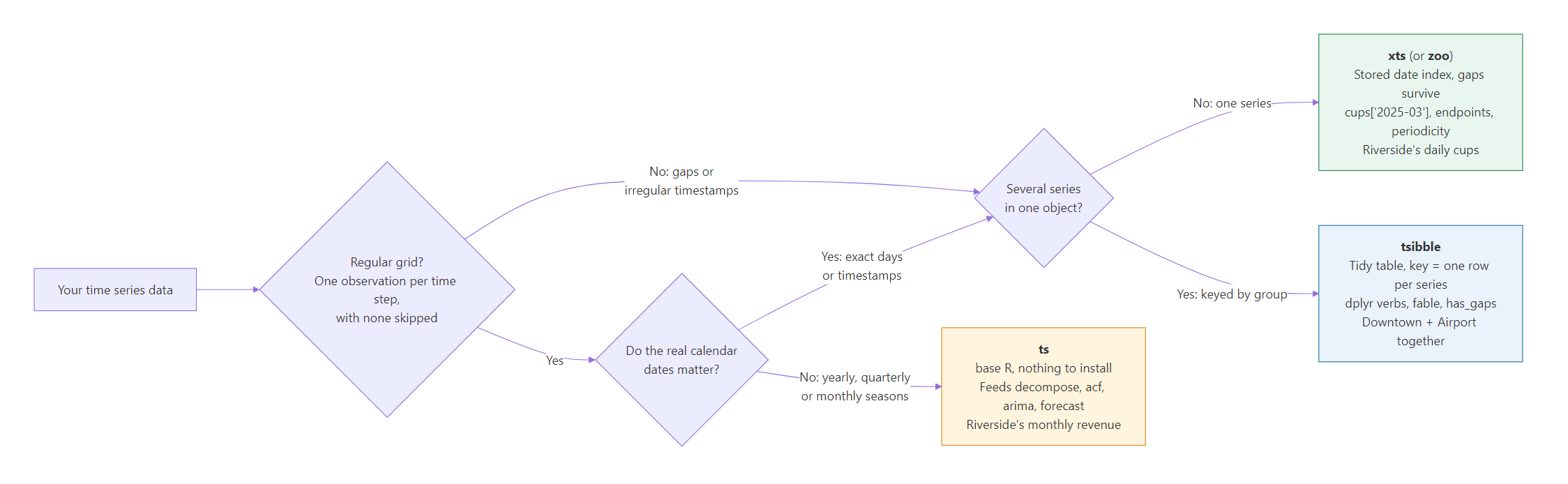
Figure 2: Three questions pick the class. Regular grid with no skipped slots and no need for exact dates goes to ts. Real dates or gaps go to xts or zoo. Several series in one object goes to tsibble.
With that settled, the choice is mechanical:
| Class | Choose it when | Riverside example | Watch out for |
|---|---|---|---|
ts |
Regular grid, seasonal period matters more than exact dates. Yearly, quarterly, monthly | Monthly revenue | Silently mis-dates any gapped data. Cannot hold a gap at all |
zoo |
Stored index, gaps allowed, index need not even be a date | Cups, if you also index by something odd | Fewer calendar conveniences than xts |
xts |
Real timestamps plus heavy calendar slicing. The finance standard | Daily cups, hourly till data | Always a matrix underneath, so it is one data type for all columns |
tsibble |
Several series in one object, tidyverse and fable workflow, gaps must be explicit |
Downtown and Airport together | Stricter: it errors on duplicate index/key rows rather than guessing |
If you are still unsure, two defaults serve well. Doing classical seasonal decomposition or ARIMA on a clean monthly or quarterly series? Use ts, it is base R and every classical function speaks it. Starting a new forecasting project, especially with more than one series? Start with tsibble, because the strictness catches problems while they are still cheap.
Continue with Time Series Analysis With R to put rev_ts through decomposition and stationarity tests, or EDA for Time Series in R to plot and profile a series before you model it.
FAQ
Do I have to pick just one class?
No, and most real projects use two or three. Converting is cheap and normal: hold your raw daily data in xts because it slices by date well, then convert to ts right before calling a classical function that demands one. Just respect the one rule above, and make the grid regular before converting to ts.
Is ts obsolete now that tsibble exists?
Not at all. ts is base R, so it needs no installation and every classical time series function in R accepts it: decompose(), acf(), arima(), HoltWinters(), and the whole forecast package. For a clean monthly or quarterly series it is the shortest path from data to model. It is the wrong tool only when your data is irregular, which is the specific failure this post walks through.
What is the difference between zoo and xts, really?
xts is a subclass of zoo, so nearly everything you know about zoo works on an xts. The differences: xts guarantees the index is a real date/time class, while zoo allows any sortable index (even letters). And xts adds the calendar tooling: date-string subsetting, endpoints(), periodicity(), to.monthly(). If your index is time, prefer xts. If it is something else you still want ordered, use zoo.
My data has gaps. Should I fill them or leave them?
It depends on what the gap means. Riverside's missing Sundays are not lost data, the shop was shut, so filling them with 0 would teach a model that Sunday demand is zero when Sunday demand does not exist. Leave those out, or mark them NA for plotting. But a gap that means "the sensor dropped out" is missing data, and there fill_gaps() plus interpolation is right. Ask whether the observation should exist. If it should and does not, fill it. If it should not, do not invent it.
I have a data frame from a CSV. How do I turn it into a time series object?
Point the constructor at the two columns, converting the date column with as.Date() first if it arrived as text: zoo(df$cups, order.by = as.Date(df$day)), or xts() with those same two arguments, or as_tsibble(df, index = day, key = shop). For ts it is ts(df$revenue, start = c(2023, 1), frequency = 12), and notice you never hand it your date column at all: ts() counts from start and ignores whatever dates you have, which is exactly the trap this post walks through. Going the other way, coredata() strips a zoo or xts back to its values and zoo::index() returns the dates; for a ts, as.numeric(rev_ts) gives the bare values and time(rev_ts) the computed index; a tsibble is already a data frame, so as.data.frame() leaves ordinary columns.
Why did my ts start at a weird date when I used frequency = 7?
Because ts counts in fractions of the frequency unit, not in dates. With frequency = 7, start = c(1, 1) means "period 1 of cycle 1", and R has no idea that cycle 1 is a particular week in your calendar. ts is happy to be abstract about this; you are the one attaching meaning. If the actual calendar dates matter to you, that is the signal to use xts or tsibble instead.
Summary
| Question | Answer |
|---|---|
| What makes an object a time series? | The index (when) is attached to the values (what) and cannot drift away from them |
How does ts store time? |
It does not. It stores start and frequency and computes the index as \(t_i = \text{start} + (i-1)/f\) |
Why does ts break on gaps? |
The formula only moves in equal steps, so "next observation" always means "one step later". A gap is unrepresentable, so it mis-dates silently, with no warning |
What do zoo and xts change? |
They store the index as a real vector, so gaps and irregular timestamps survive. index() and coredata() split the halves |
What does xts add over zoo? |
A guaranteed date/time index plus calendar tooling: x["2025-03"], endpoints(), periodicity() |
What does tsibble add? |
The index lives in a column and a key column separates several series in one tidy table. It detects and reports gaps rather than hiding them |
| Which conversions are lossy? | Converting to ts from an irregular index destroys the dates. Converting away from ts is always safe |
| What does "regular" actually mean? | One observation per time step with none skipped. Not "all day-gaps equal": monthly data has 28 to 31 day gaps and is perfectly regular |
Riverside Roasters needed two different answers, which is the honest conclusion of the whole comparison. Its monthly revenue is a clean regular grid where exact dates do not matter, so ts is right. Its daily cups have a real hole every Sunday, so ts is wrong, and xts (or tsibble, once the Airport shop opened) is right. Same business, same analyst, different classes, chosen on one question: is there a time step the data should have and does not?
References
- zoo: An S3 Class and Methods for Indexed Totally Ordered Observations - the package vignette by Zeileis and Grothendieck. The clearest statement of the stored-index design and why it exists.
- Introduction to xts and zoo - the xts vignette. Read it for the date-string subsetting and
endpoints()sections. - xts package documentation - Joshua Ulrich's reference site, with the full function index and the period-apply family.
- tsibble: Tidy Temporal Data Frames - the official tsibble site. The "Introduction to tsibble" article covers index, key and gap handling properly.
- Forecasting: Principles and Practice, chapter on tsibbles - Hyndman and Athanasopoulos. The canonical free text; this chapter motivates tsibble from a forecasting point of view.
- R documentation: ts() - the base R manual page. The definitive statement of what
start,frequencyanddeltatmean. - CRAN Task View: Time Series Analysis - the maintained map of the whole R time series ecosystem, organised by task.
Continue Learning
- Time Series Analysis With R is the natural next step. It takes a
tslikerev_tsand decomposes it into trend, seasonality and remainder. - EDA for Time Series in R covers the plots and checks to run on a series before modelling it.
- Time Series Forecasting With R picks up where the objects end, turning a correctly classed series into a forecast.
- Time Series Exercises in R has practice problems if you want to drill the conversions.