Calendar Effects in R: Trading Days, Holidays, Time-Zone Traps
A calendar effect is a movement in a time series caused purely by how the calendar happens to fall, different numbers of working days per month, holidays that shift date each year, and clocks that jump forward and back, rather than by any real change in the activity you are measuring. Left alone, these effects get baked into your seasonal estimates and your forecasts inherit the error.
What is a calendar effect, and why does it wreck a forecast?
Here is the cleanest way to feel the problem. Build one year of daily activity with no trend, no seasonality, and no randomness at all: every weekday earns exactly 100, every weekend earns exactly 0. Then add the days up by month, which is what almost every reporting system does.
Walking through the code: seq() lays out all 366 days of 2024, wday(days, week_start = 1) numbers Monday as 1 through Sunday as 7 so the <= 5 test picks out weekdays, and floor_date(date, "month") snaps every date back to the first of its month so group_by() can total them.
Now read the output. June says 2000 and January says 2300. Nothing about the business changed between those two months. June 2024 simply contained 20 weekdays and January contained 23. That gap is entirely an artefact of where the weekends happened to fall in 2024.
A 13.7% peak-to-trough swing, in a series that by construction contains no information whatsoever. If you handed this to auto.arima() or an ETS model, the two standard automatic forecasting methods, it would estimate a seasonal pattern from those numbers, and that pattern would be wrong the moment the calendar shifted in a later year.
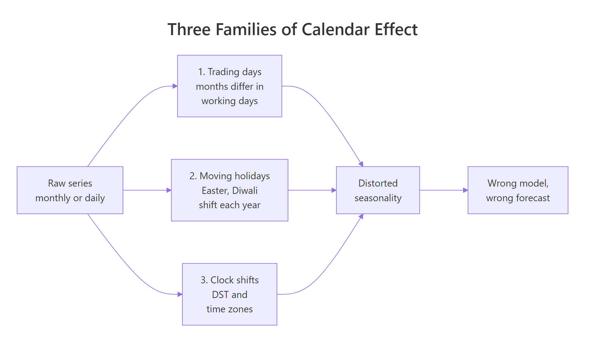
Figure 1: The three families of calendar effect and the single failure they all lead to.
The diagram splits the problem into the three families you will meet. Trading days are the one you just saw: months contain different numbers of working days. Moving holidays are festivals like Easter or Diwali that land on a different date each year, so they migrate between months. Clock shifts are daylight saving transitions and time zone mistakes, which quietly change how many hours a "day" contains. The rest of this tutorial handles each in turn, and every technique here is plain lubridate and dplyr, so nothing depends on a specialist calendar package.
Try it: Work out which month of 2026 has the fewest weekdays and which has the most. Build the daily grid for 2026, count weekdays per month, then keep only the rows matching the minimum or the maximum.
Click to reveal solution
Explanation: February 2026 offers 20 weekdays while July and December offer 23. That is a 15% spread before a single customer has done anything, and it is why raw month-on-month comparisons mislead.
How do you count trading days in R?
Everything in this tutorial is built on one function, so it is worth getting it exactly right. wday() turns a date into a day-of-week number, but its default numbering catches almost everyone out.
By default R follows the US convention where Sunday is day 1 and Saturday is day 7. That means the natural-looking test wday(x) <= 5 selects Sunday through Thursday, which is wrong nearly everywhere. Passing week_start = 1 switches to the ISO convention where Monday is 1 and Sunday is 7, and then <= 5 really does mean Monday to Friday.
Three columns, three jobs. wday_no is the raw number you compute with, wday_lb adds label = TRUE to get a readable ordered factor you can filter on by name, and weekday is the logical flag that does the actual work. Monday came back as 1, Sunday as 7, and weekday is TRUE for the two weekdays and FALSE for the weekend, exactly as intended. Always sanity-check this on dates whose weekday you already know before trusting a count built on top of it.
With the convention pinned down, counting weekdays per month is a two-line summarise. This is your first real calendar regressor, and the word is worth pinning down too: a regressor is simply an extra column you hand to a model as an explanatory variable. Here that column holds one number per month, the count of weekdays that month contained.
The trick that makes this work is sum() on a logical vector. R treats TRUE as 1 and FALSE as 0, so summing the is_weekday flag counts how many days passed the test. That pattern, flag each day then sum the flag, is the engine behind every regressor in this tutorial.
Compare this column against the sales table from the previous section and they match perfectly: 23 weekdays gave 2300, 20 weekdays gave 2000. You have now explained 100% of that phantom seasonality with a single number per month.
Try it: Not all weekdays are equally common. Count how many Fridays fall in each month of 2025. Filter the daily grid down to Fridays, then count by month.
Click to reveal solution
Explanation: Because label = TRUE returns a factor, you can filter by the readable name "Fri" instead of remembering that Friday is number 5. Four months of 2025 contain five Fridays and eight contain four. If Friday is your biggest trading day, that difference alone moves monthly revenue by several percent, which is exactly the effect the seven-regressor approach later in this tutorial is designed to capture.
How do you build a holiday calendar without a specialist package?
Weekends are easy because they repeat on a fixed weekly cycle. Holidays are harder, and they come in two flavours. Some sit on a fixed date every year, like Christmas on 25 December. Others are defined by a rule, like "the fourth Thursday of November". The rule-based ones are where people reach for a package, and they do not need to.
The trick is to notice that the nth occurrence of a weekday within a month is pure arithmetic on the day-of-month number. The first Monday of a month always falls on day 1 to 7, the second on day 8 to 14, and so on. So ceiling(mday / 7) tells you which occurrence you are looking at, whatever the weekday. The mirror-image test for the last occurrence asks whether another day of the same weekday would still fit inside the month. Adding 7 days to it would run past the end, so the test reduces to checking that the date sits in the final seven days of the month.
The output shows all four Thursdays in November 2024 with their nth labels running 1, 2, 3, 4. The 28th is both the fourth Thursday and the last one, so is_last is TRUE there and FALSE everywhere else.
That single grid now answers every "nth weekday of the month" question by filtering, with no loops and no date arithmetic.
Two filters, six correct dates across three years. pull() just extracts the date column as a plain vector so the output is easy to read.
Fixed-date holidays bring their own wrinkle. When Christmas or Independence Day lands on a weekend, most employers shift the day off to the nearest weekday. The convention in the United States is that a Saturday holiday is observed on the preceding Friday and a Sunday holiday on the following Monday.
The nested ifelse() adds minus one day for a Saturday, plus one day for a Sunday, and zero otherwise. Because ifelse() is vectorised, the function handles a whole column of dates at once.
The result covers all three cases in one table. 2026 shifts back to Friday the 3rd, 2027 shifts forward to Monday the 5th, and 2028 already falls on a Tuesday so nothing moves. Getting this right matters more than it looks, because when a holiday sits next to a month boundary the shift carries it across. 1 January 2028 falls on a Saturday, so the day off is taken on Friday 31 December 2027, which puts the lost trading day in a different month and a different year from the holiday itself.
Now assemble both halves into one reusable function.
The function rebuilds the grid for whatever years you ask for, pulls the five fixed dates and pushes them through observed(), pulls the six rule-based ones, then sort(unique(...)) merges the two vectors and removes any overlap.
Eleven dates come back for 2025, which is the correct count for US federal holidays. Spot-check a couple: 20 January is the third Monday, and 26 May is the last Monday of May. You now have a holiday calendar you fully control and can adapt to any country by editing two filters.
Moving festivals are the last piece, and Easter is the one that matters most for European and Latin American series. Its date is set by a lunar rule, so it can land anywhere between 22 March and 25 April. The standard closed-form solution is the anonymous Gregorian computus, and it is plain arithmetic.
You do not need to follow the modular arithmetic, it is a published algorithm and every operator here is %% (remainder) or %/% (integer division) applied to whole vectors at once. Feed it a vector of years and it returns a vector of dates.
The dow column returning Sunday five times out of five is your correctness check, since Easter is Sunday by definition. Look at what the month column does though: 2024 and 2027 put Easter in March, the other three years put it in April. For a monthly retail series that single fact moves an entire holiday's worth of trade between two months, and no fixed seasonal factor can absorb it.
For US financial data specifically, exchange calendars differ from federal ones. The timeDate package ships them, and comparing it against what you just built is instructive. This block needs a local R session rather than the browser.
# Run this locally in RStudio: timeDate is not available in the browser
library(timeDate)

nyse <- as.Date(holidayNYSE(2025))
nyse
#>  [1] "2025-01-01" "2025-01-20" "2025-02-17" "2025-04-18" "2025-05-26"
#>  [6] "2025-06-19" "2025-07-04" "2025-09-01" "2025-11-27" "2025-12-25"

length(nyse)
#> [1] 10
Compare that list against your federal one and two differences jump out. The NYSE closes on Good Friday (18 April 2025), which is not a federal holiday at all. It stays open on Columbus Day and Veterans Day, which are federal holidays. Ten dates against eleven, and only nine of them overlap.
Try it: Labor Day in the United States is the first Monday of September. Use the nth trick to find it for 2025, 2026 and 2027.
Click to reveal solution
Explanation: Three filters stack up to define the rule exactly as it is written in law: September, Monday, first occurrence. Note how far the date moves, from the 1st in 2025 to the 7th in 2026. That six-day drift is enough to shift a long weekend's trade out of one week and into another.
How do you feed the calendar into a forecasting model?
You now have the ingredients. The next step is turning them into a column your model can use, which means counting trading days properly (weekdays that are not holidays) and attaching that count to a time series object.
The workflow below is the one worth memorising, because the last step is where most people come unstuck.

Figure 2: Turning a raw calendar into a model regressor, and the future-values step people forget.
Start by flagging every day in a long span, well past the end of your data, then aggregating to the series frequency. Building the calendar out into the future costs nothing now and saves you at forecast time.
Two things changed from the earlier weekday count. The is_trading flag now has a second condition, !(date %in% hols), which excludes any date appearing in the holiday vector. And yearmonth() from tsibble replaces floor_date(), producing the monthly index type that tsibble and fable expect.
The 2025 numbers run from 18 to 22. November is the low month because it loses Veterans Day and Thanksgiving on top of having only 20 weekdays. That is a 22% spread between the best and worst month of a single year, which no seasonal factor fitted on other years will reproduce.
Next, build a monthly series and attach the regressor. The simulated series below has a real upward trend and a genuine December uplift, plus the trading-day effect, so there is something for the model to actually separate.
Reading the construction: multiplying by is_trading zeroes out closed days, trend_part adds a slow rise of about 0.02 per day, dec_boost adds a genuine December lift, and rnorm() supplies noise. The left_join() then glues the regressor column on, and as_tsibble(index = month) declares which column is time.
The printed header [1M] confirms tsibble recognised a monthly series. Each row now carries both the value and the number of trading days that produced it, which is exactly what a regression model needs.
Now the payoff. Fit two models on the same data, one that only knows about trend and month-of-year, and one that also sees the trading-day count.
TSLM() is fable's time series linear model. trend() inserts a straight-line time index and season() inserts eleven monthly dummy variables, so plain is the standard textbook specification. The calendar model is identical plus one extra column. glance() then pulls out the fit statistics for both.
The difference is not marginal. Residual variance (sigma2) falls from 13098 to 1738, a factor of 7.5. AICc is a model-comparison score that rewards fit and penalises extra parameters, and lower is better, so a drop of 168 points is a large win rather than a rounding difference. One column did all of that, because the eleven seasonal dummies were trying to capture something that genuinely changes from year to year, and a fixed dummy per month cannot.
This is the most informative output in the tutorial, so read it carefully. n_trading has an estimate of 131.34 with a t value of 21.6, meaning each extra trading day is worth about 131 units of sales and the evidence for it is overwhelming.
Now look at the seasonal dummies. Months 2 through 11 are all statistically indistinguishable from zero, with p-values from 0.07 to 0.76. Only season()year12 survives, at 621, which is the genuine December uplift that was built into the data. The model has correctly separated the two: real seasonality lives in the December dummy, and the calendar noise lives in n_trading.
Here is the step the workflow diagram flagged at its end. A model with an external regressor cannot forecast from a horizon alone, because it has no idea what n_trading will be next March. Ask for six steps ahead and it stops.
tryCatch() catches the error instead of halting, and grep() picks out the two informative lines from fable's message. The complaint is precise: it needs n_trading and cannot invent it.
This is the single most common stumble when moving from TSLM(y ~ trend() + season()) to a model with real predictors, and the error message is honest about the cause. The fix is to supply the future calendar, which you already built.
Because td_month was built all the way to the end of 2026, the future values are just a filter away. This is why the earlier advice to extend the calendar past your data pays off.
Notice that these are not forecasts. The number of trading days in March 2026 is a known fact, fixed by arithmetic. That certainty is precisely what makes calendar regressors so useful: unlike most predictors, you never have to forecast them first.
Swapping h = 6 for new_data = future_cal gives fable both the horizon and the regressor values in one object, so it forecasts happily.
Look at the relationship between the two columns. February is forecast lowest at 2944 with 19 trading days, March and April highest at around 3337 with 22. The forecast is now tracking the actual shape of 2026's calendar rather than assuming next February will resemble an average February.
Try it: Fit a model with n_trading on sales_month and read off just that coefficient. Use tidy() to get a tidy coefficient table, then filter to the term you want.
Click to reveal solution
Explanation: tidy() turns a fitted model into a data frame with one row per coefficient, which is far easier to filter than reading a printed summary. The 131 matches the report() output above, and it has a directly useful business reading: gaining one trading day is worth roughly 131 units.
Why do seven day counts beat one trading-day total?
A single trading-day count assumes every working day is worth the same. For an office that is roughly true. For a restaurant, a cinema or a supermarket it is badly false, because Saturday might do triple Monday's business while Sunday sits somewhere in between.
The fix, which comes from the official seasonal adjustment literature, is to replace one count with seven: how many Mondays, how many Tuesdays, and so on. Building them is a count() plus a reshape.
count() gives one row per month-weekday combination, and pivot_wider() spreads the dow values into seven columns with the counts as values. Ten years of history gives the model enough variation to work with, which matters here more than usual.
Every month has either four or five of each weekday, and which weekdays get the extra one rotates. January 2016 had five Fridays, Saturdays and Sundays; February 2016 had five Mondays instead. For a weekend-heavy business those two months are not comparable at all.
Now build a series where weekends genuinely dominate, and pit one regressor against seven.
The weights vector sets each weekday's true daily value, and indexing it by as.character(dow) looks up the right one for every date. The - 1 in the second formula drops the intercept, which is necessary because the seven counts already add up to the length of the month and would otherwise be perfectly collinear with it.
Residual variance falls from 14078 to 1053, a factor of 13, and AICc drops by 305 points. The total-days model knew February was short but had no way to know whether it was short of Saturdays or short of Tuesdays, and for this business those are very different things.
Adding a truth column by looking up the same weights vector lets you grade the model directly, which you can only do with simulated data but which is the fastest way to build trust in a technique.
Every estimate lands within roughly one standard error of the value used to generate the data. Saturday comes back at 266 against a truth of 260, Monday at 88 against 80. The model has recovered the entire weekly profile from nothing but monthly totals and day counts, which is a genuinely surprising amount of information to extract from twelve numbers a year.
Try it: Confirm the weekend story by ranking the coefficients. Sort the seven-day model's estimates from largest to smallest and show the top three.
Click to reveal solution
Explanation: arrange(desc(estimate)) sorts largest first. The weekend plus Friday take the top three slots, and Saturday alone is worth about three Mondays. A month that happens to contain five Saturdays instead of four gains roughly 266 units for reasons that have nothing to do with demand.
What breaks when the clock changes?
Everything so far worked in whole days, where a date is unambiguous. Move to hourly or sub-daily data and a new class of bug appears, because the relationship between "clock reading" and "moment in time" stops being one-to-one twice a year.
Two lubridate functions handle the conversion between them, and they do opposite things. Mixing them up is the most common date-time bug in R.
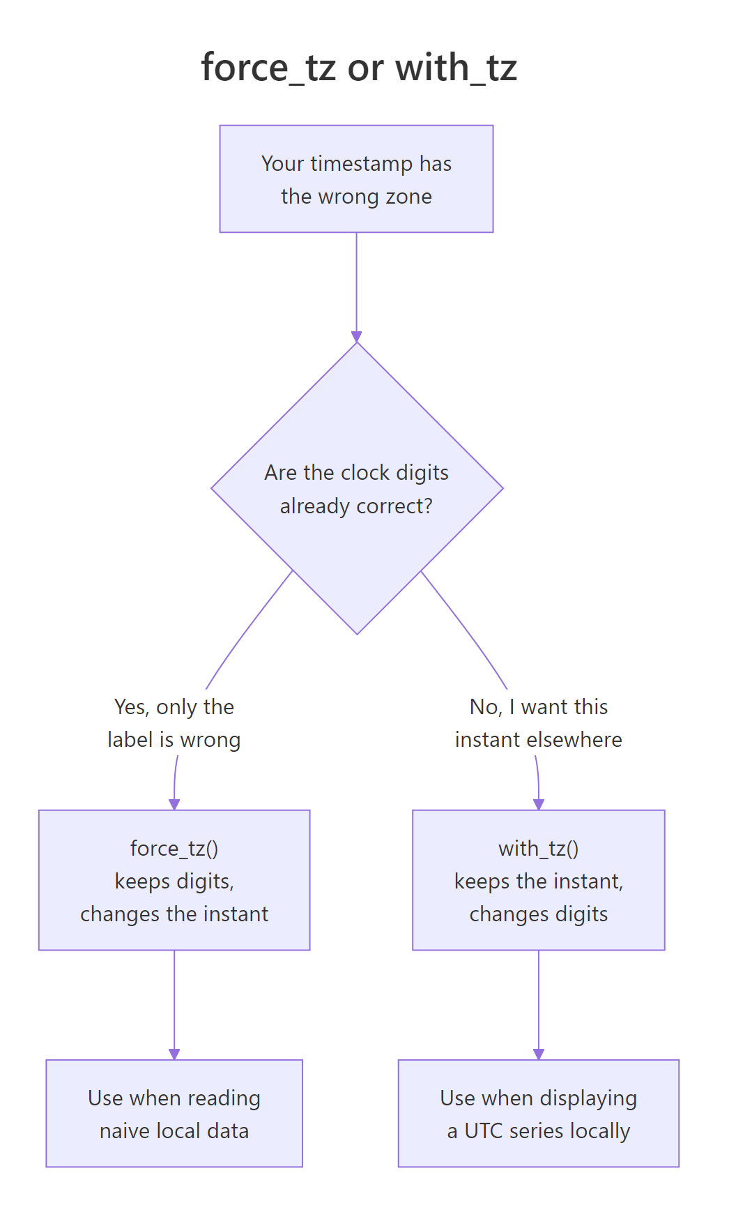
Figure 3: Choosing between force_tz() and with_tz().
The distinction is worth stating plainly before you see the code. A timestamp carries two pieces of information: an instant (a specific moment in the history of the universe) and a clock reading (the digits a local wall clock would show). force_tz() keeps the digits and changes the instant. with_tz() keeps the instant and changes the digits.
Same input, two very different outputs. force_tz() still reads 09:00 but it is now a New York morning, four hours later in real time than the UTC original. with_tz() still refers to the identical moment, but expressed in New York it reads 05:00.
The practical rule: use force_tz() when your data arrived as naive local timestamps that R wrongly labelled UTC on import, and use with_tz() when you have correct instants and want to display or aggregate them in someone's local time.
Now the part that silently destroys data. On the spring-forward night the local clock jumps straight from 02:00 to 03:00, so 02:30 never existed.
Rather than inventing a plausible instant, lubridate returns NA and warns. That is the right behaviour, but a warning in the middle of a long import script is easy to miss, and you end up with a hole in the series that surfaces much later as a mysterious gap.
The autumn transition creates the opposite problem. When the clock falls back, 01:30 happens twice, once on daylight time and once an hour later on standard time.
No warning at all this time. Lubridate silently resolved the ambiguity by picking the standard-time occurrence, shown by the EST label and confirmed by the 06:30 UTC conversion (the daylight-time reading would have been 05:30 UTC).
That is a full hour of error, applied silently, on one day a year. If your data source recorded the first occurrence instead, every value in that hour is now attributed to the wrong hour.
Arithmetic has its own version of the trap. Adding "a day" can mean two different things, and lubridate makes you choose.
days(1) is a period, meaning "the same time tomorrow", so it lands on noon regardless of what the clock did overnight. ddays(1) is a duration, meaning exactly 86400 seconds, and because 10 March lost an hour it overshoots to 13:00.
Neither is wrong. Business logic ("the shop opens at noon tomorrow") wants days(1). Physical measurement ("24 hours of exposure") wants ddays(1). Choosing by accident is what causes trouble, and the default habit of writing + 86400 always gives you the duration behaviour whether you wanted it or not.
The consequence for aggregation is that days are not all the same length. Generate hourly timestamps across the spring transition and count them.
seq() steps hour by hour through local time and count() tallies how many landed on each date. Ten March got 23 rows because the 02:00 hour does not exist in that zone.
The autumn transition does the reverse.
Twenty-five hours on 3 November. Now think about what a daily sum() does to that: energy load, web traffic and call volumes all get a free 4% bump on one day each autumn and a 4% dip each spring, purely from clock arithmetic. Every anomaly detector you run will flag both.
Try it: Confirm the effect on a different year. Count the hourly observations per day between 8 and 10 March 2025 in New York, and find the short day.
Click to reveal solution
Explanation: In 2025 the transition fell on 9 March rather than 10 March, because the rule is "the second Sunday in March" and that is a rule-based date exactly like the holidays earlier. The short day moves every year, so hard-coding last year's date will not protect you.
Which time zone should your time series live in?
The previous section showed what goes wrong. This one gives you the policy that prevents it, and it comes down to three decisions made in the right order.
First, understand why a naive timestamp string is not enough information. The same text, read in three different zones, is three genuinely different moments.
sapply() runs the same conversion for each of the three zone names: interpret the string in that zone with as.POSIXct(tz = z), then express the result in UTC so all three are directly comparable.
Thirteen hours separate the New York and Tokyo readings of the identical text. Worse, as.POSIXct() with no tz argument at all does not fail, it silently uses whatever zone the machine is configured for. The same script then produces different numbers on your laptop, your colleague's laptop and the production server.
The middle step of that rule deserves a demonstration, because it is where judgement is actually required. Take the same hourly instants from the previous section and count them by UTC date instead of local date.
Every full day in the middle now has exactly 24 hours, DST transition or not. The partial 19 and 4 at the ends are just the five-day local window straddling six UTC dates, which is the offset at work rather than a bug.
So which is right? It depends on what the data measures. Electricity demand, retail footfall and app usage follow human routines, so they belong on local days even though those days are ragged. Server throughput, sensor readings and anything physical belongs on UTC days, where every day really is 24 hours long. Choose deliberately, then write the choice into the code as a comment, because the two produce different answers and both look reasonable.
Try it: Take the ex_hours object from the previous exercise and recount it by UTC date instead of local date, then compare the row count.
Click to reveal solution
Explanation: The 23-hour day has vanished. In UTC, 9 March 2025 has a full 24 hours because UTC never observes daylight saving. Three local dates became four UTC dates, which is the five-hour offset splitting the window differently, not lost or duplicated data. The totals still match: 71 observations either way.
Complete Example
Time to put the whole toolkit to work on one realistic problem. You have eight years of daily revenue for a US business that closes at weekends and on federal holidays. The question is whether a calendar regressor measurably improves a forecast, tested honestly on data the model never saw.
The plan is: build a holiday-aware trading-day calendar running past the end of the data, aggregate revenue to months, train on 2018 through 2024, test on 2025, and compare a plain seasonal model against a calendar-aware one.
Following the pipeline: calendar runs to the end of 2026 so future values are ready, revenue simulates daily takings with a trend and a December uplift then rolls up to months, train and test split at the end of 2024, and accuracy() scores both models' 2025 forecasts against what actually happened.
The verdict is decisive. Mean absolute percentage error falls from 3.58% to 1.18%, and root mean squared error from 6684 to 2499. The calendar model's typical monthly forecast error is less than a third of the plain model's, from one extra column that required no forecasting of its own.
With the better model chosen on evidence, produce the forecast that the business actually asked for.
The filter() slices the pre-built calendar down to the forecast window, and round() tidies the output for reporting.
The forecast tells a story a plain model could not. February 2026 is the weakest month at 147k, but not because February is inherently weak, it is because 2026 gives it only 19 trading days. If the business compares February against March and sees a 17k gap, the calendar explains almost all of it, and nobody needs to launch an investigation into a sales slump that never happened.
Practice Exercises
Exercise 1: Build an Easter regressor split across months
Easter moves between March and April, so a monthly series needs its effect apportioned between the two. The standard method treats the holiday as a window of days and gives each month the fraction of that window it contains.
Build a regressor for 2018 to 2025 using a 7-day window ending on Easter Sunday (the six days before, plus Easter itself). For each month that overlaps a window, report how many of the 7 days fell in it and what share of the window that is. You will need the easter_date() function from earlier in the tutorial.
Click to reveal solution
Explanation: rep(my_easter, each = 7) repeats each Easter date seven times, and subtracting rep(6:0, ...) walks backwards from six days before to Easter itself. count() then does the apportioning automatically, because days that crossed a month boundary land in different yearmonth() groups.
Read the interesting years. 2018 splits 6 days into March and 1 into April; 2021 splits 3 and 4. The other six years fall entirely within one month. That easter_share column is what you feed to TSLM() as a regressor, and it is the same logic the US Census Bureau's genhol function implements for X-13ARIMA-SEATS.
Exercise 2: Decide which series has a trading-day effect
You are handed two monthly series and asked which one needs a calendar adjustment. Guessing from a plot is unreliable because a trading-day effect looks a lot like ordinary seasonality.
Build both series with the code below, then regress each on n_trading and use the coefficient's t statistic and p-value to decide. Reshape to long form and use a keyed tsibble so one model() call handles both. Expect a t statistic above 10 for the series that has an effect and below 2 for the one that does not.
Click to reveal solution
Explanation: Reshaping to long form and declaring key = series makes a keyed tsibble, so a single model() call fits one model per series and tidy() returns both coefficient sets stacked with a series column.
The answer is unambiguous. Series A has a t statistic of 13.9 and a p-value near zero, so it needs a trading-day regressor. Series B has t = -0.83 and p = 0.41, which is exactly what noise looks like, so adding the regressor there would only cost a degree of freedom. Series B was built from a trend plus noise with no calendar dependence at all.
Exercise 3: Aggregate hourly data safely across a DST transition
An energy team gives you hourly load readings across the November fall-back weekend and asks for daily figures. The readings are deliberately constant at 100 for every single hour, so any variation you see in the daily output is an artefact and not a signal.
Build the hourly frame below, then group by local date and report three things per day: the number of observations, the sum of load, and the mean of load. Then explain which of sum() and mean() you would ship to the energy team, and why.
Click to reveal solution
Explanation: The n_obs column is the tell: 3 November carries 25 readings because the 01:00 hour occurred twice. The total column duly reports 2500 against 2400 on the neighbouring days, a 4.2% spike, even though the load never changed by a single unit. The average column stays flat at 100, which is the truth.
Ship the mean, or ship the sum with n_obs beside it so the reader can normalise. Shipping a bare daily sum guarantees that one day every autumn looks like a demand surge and one day every spring looks like an outage, and both will be investigated by someone who does not know about clocks.
Frequently Asked Questions
Why not just divide the monthly total by the number of trading days?
That is the obvious alternative and it does remove most of the distortion, but it forces the effect to be exactly proportional: 5% more trading days must mean 5% more sales. A regressor lets the model estimate the per-day value from the data instead of assuming it, which matters when part of the month's activity is fixed (a subscription base, a standing order) and does not scale with opening days at all. Dividing also destroys the units of the series, so your forecast comes back as "sales per trading day" and has to be multiplied out again.
Does a weekly or daily series need this too?
A weekly series is the one case that mostly escapes, because every week contains exactly seven days and one of each weekday, so there are no trading-day counts to vary. It still needs holiday handling, since a public holiday inside a week is a genuine loss. Daily series have the opposite problem: the day-of-week pattern is not a nuisance count any more, it is the seasonality itself, so you model it directly with a weekly seasonal term plus holiday dummies rather than with the monthly counts built here.
What about leap years and months of different lengths?
Month length is handled automatically, because counting weekdays or trading days per month already absorbs it. February 2024 gets 20 trading days and February 2025 gets 19, and the extra one is the leap day itself, 29 February 2024, which happened to fall on a Thursday. n_trading carries that difference without any extra work. The only place you have to think about it separately is the is_last test, which is why the code calls days_in_month(date) instead of hard-coding 30 or 31.
Should I use a package like timeDate or bizdays instead of writing this myself?
Use a package when it already ships the exact calendar you need, which is the case for major exchanges (timeDate::holidayNYSE()) and for the financial centres covered by bizdays. Build it yourself when your calendar is company-specific, regional, or simply not in any package, which covers most real business series: a warehouse that shuts for a local festival, a clinic with its own closure days. The grid pattern in this tutorial is worth knowing either way, because it is what lets you edit a packaged calendar rather than accept it.
One trading-day count or seven day-of-week counts?
Start with one count and only move to seven if the business genuinely trades at different rates on different days. Seven regressors need roughly five years of monthly data before the coefficients settle, because each count only ever takes the value 4 or 5. A useful middle option when history is short is two columns, weekday count and weekend-day count, which captures most of the retail pattern at a quarter of the parameter cost.
Do auto.arima() or ETS handle calendar effects on their own?
No. Both estimate a fixed seasonal pattern, meaning one factor for January that is reused for every January, so a January with 23 trading days and a January with 21 get the same adjustment. That is exactly the assumption calendar effects violate. The fix is to pass the calendar in as an external regressor, which ARIMA supports through ARIMA(y ~ n_trading + pdq(...)) in fable; ETS does not accept external regressors at all, so a calendar-sensitive series is a reason to prefer a regression or ARIMA model over ETS.
Summary
Calendar effects are not exotic. They show up in any series aggregated to a period the calendar does not divide evenly, which is nearly all of them.
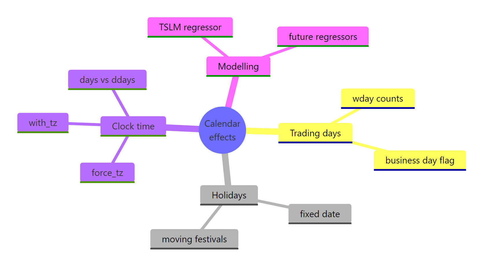
Figure 4: The calendar-effects toolkit at a glance.
| Effect | How it shows up | Fix in R |
|---|---|---|
| Trading days | Monthly totals swing 10-15% with no real change | Count working days per month, add as a regressor |
| Holidays | Certain months dip for reasons no seasonal factor explains | Build a holiday vector, exclude those dates from the count |
| Observed shifts | A holiday's cost lands in the wrong month | Shift Saturday holidays to Friday, Sunday to Monday |
| Moving festivals | March and April swap places year to year | Compute the date (Easter computus), split the window across months |
| Unequal weekdays | Weekend-heavy business, one total count underfits | Use seven day-of-week counts instead of one |
| DST transitions | One day has 23 hours, another has 25 | Aggregate with mean(), or store the observation count |
| Time zone drift | Same script, different answers on different machines | Store UTC, aggregate local, display local |
The key techniques, in the order you will reach for them:
wday(x, week_start = 1)so Monday is 1, otherwise every count is off by a day per week.nth = ceiling(mday(x) / 7)andis_last = mday(x) > days_in_month(x) - 7to express any "nth weekday of the month" holiday as a filter.sum(logical_column)to turn per-day flags into per-period counts.TSLM(y ~ trend() + season() + n_trading)to let seasonality and the calendar each do their own job.forecast(new_data = ...), neverh = ..., once a model has an external regressor.force_tz()versuswith_tz(), decided by whether the digits or the instant is the thing that is already correct.
The single most valuable habit is building the calendar past the end of your data. Future trading-day counts are arithmetic, not forecasts, so they cost nothing to compute and they are the one predictor you will never be uncertain about.
References
- Hyndman, R.J. & Athanasopoulos, G. Forecasting: Principles and Practice, 3rd Edition. Section 7.4: Some useful predictors (trading days, Easter, distributed lags). Link
- Monsell, B.C., Issues in Modeling and Adjusting Calendar Effects in Economic Time Series. US Census Bureau, Proceedings of ICES-III (2007). Link
- Sax, C. & Eddelbuettel, D., Seasonal Adjustment by X-13ARIMA-SEATS in R. Journal of Statistical Software. Covers the
genhol()function for moving-holiday regressors. Link - lubridate reference, time zone functions
force_tz(),with_tz(), and the period versus duration distinction. Link - fable reference,
TSLM()and forecasting with external regressors vianew_data. Link - Wang, E., Cook, D. & Hyndman, R.J., A New Tidy Data Structure to Support Exploration and Modeling of Temporal Data. Journal of Computational and Graphical Statistics (2020). The tsibble paper. Link
- timeDate package,
holidayNYSE()and other exchange calendars. Link - IANA Time Zone Database, the authoritative source behind every Olson zone name such as
America/New_York. Link - R Core Team, An Introduction to R, and the
?as.POSIXcthelp page on the empty time zone default. Link
Continue Learning
- Time Series Regression in R goes deeper on
TSLM(), including the spurious regression trap and how to check residual assumptions once you have added regressors like the ones built here. - tsibble in R explains the tsibble object model used throughout this tutorial: index columns, keys for multiple series, and how to find and fill gaps in irregular data.
- Dates and Times Drills in R is fifteen graded problems on parsing, arithmetic and time zones, and is the fastest way to make the lubridate patterns here automatic.