Time Series Decomposition in R: STL vs Classical
Time series decomposition splits one messy series into three readable parts: a trend-cycle (the long-run level), a seasonal component (the pattern that repeats each cycle), and a remainder (whatever is left over). This tutorial builds both classical decompose() and stl() from scratch in base R, on real data, and shows you exactly when to reach for each. Nothing to install.
What is time series decomposition, and why split a series apart?
Picture monthly airline ticket sales. Three forces push the number around at the same time. The business is growing year over year, every summer brings a travel spike, and the odd month lands above or below what those two forces alone would predict. Read together they blur into one jagged line. Decomposition pulls them apart so you can study each force on its own.
R ships with the perfect example built in. AirPassengers records the monthly total of international airline passengers from 1949 to 1960. One function call, decompose(), splits it apart. It returns a list, and one slot of that list is named figure: the twelve monthly seasonal factors it worked out. Print them.
Those twelve numbers describe the repeating yearly pattern of air travel, one factor per month from January to December. July sits at 1.227, meaning traffic runs about 23 percent above the year's underlying level, while November's 0.801 is roughly 20 percent below it. In one line you have already learned when planes fill up. We passed type = "multiplicative" because this series' seasonal swing grows as the airline grows, and you will see exactly why in a moment.
decompose() gave back more than the seasonal shape. It also returns a trend-cycle and a remainder, and the clearest way to meet all three is to plot them together.
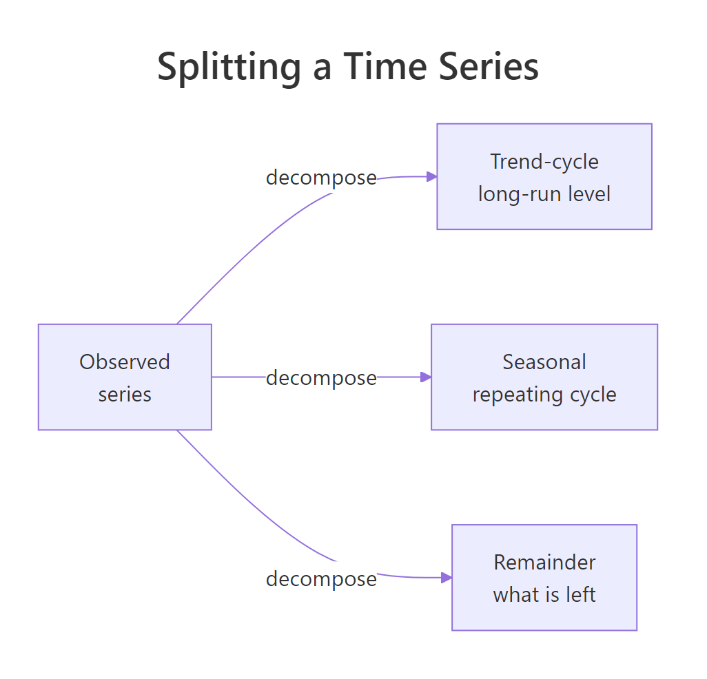
Figure 1: One observed series splits into a trend-cycle, a seasonal component, plus a leftover remainder.
The chart stacks four panels. The top one is the original tangled series. Below it sit the three parts decomposition pulled out: a smooth trend climbing from the late 1940s, the repeating seasonal wave, and a thin remainder of leftover noise. One jagged line has become three clean stories you can read separately. Everything that follows is about understanding those panels and choosing the right method to build them.
AirPassengers is stored as an R time series (a ts object) that knows it is monthly with 12 observations per cycle, so decompose() never has to be told the season length. When you build your own series with ts(x, frequency = 12), that frequency argument is what makes seasonal decomposition possible.Try it: The nottem dataset holds 20 years of monthly air temperatures at Nottingham Castle. Plot it and see which of the three forces (trend, season, noise) your eye can spot.
Click to reveal solution
Explanation: nottem shows a large, regular seasonal wave (hot summers, cold winters) but almost no upward or downward drift, so its trend is nearly flat. That contrast with AirPassengers matters later when we choose a model.
What are the trend, seasonal, and remainder components?
You have met the seasonal factors already. The components object is a list, and the other two parts live in their own slots. Let's open them so the panels stop being abstract. First the trend-cycle, the smooth backbone left once the yearly wave and the noise are stripped away.
Two things stand out. The trend for 1949 rises gently from about 127 to 130, which is the underlying level once the summer spike is removed. And the first six months are NA. That is not a bug. Classical decomposition estimates the trend with a moving average that needs six months of data on each side, so it cannot reach the very start of the series. Hold that thought, it becomes a real limitation later.
Whatever the trend and season together cannot explain lands in the remainder.
The remainder is centered near 1 in a multiplicative model. A value of 0.952 for July 1949 means that, after accounting for the trend and the usual July bump, actual traffic came in about 5 percent lower than expected. Small, patternless wobbles like these are exactly what you want here. Structure left behind in the remainder (a visible wave, a drift) is a warning that the model missed something.
Try it: Find the busiest travel month by locating the largest seasonal factor. Use which.max() and translate the position into a month name with the built-in month.abb vector.
Click to reveal solution
Explanation: which.max() returns the position of the biggest value (7), and month.abb[7] maps that position to "Jul". July is the peak of the summer travel season.
Should you use an additive or multiplicative model?
Every decomposition rests on one modeling choice: how do the three parts combine? There are two answers. In an additive model the parts add up, and in a multiplicative model they multiply.
$$y_t = T_t + S_t + R_t \qquad \text{(additive)}$$
$$y_t = T_t \times S_t \times R_t \qquad \text{(multiplicative)}$$
Where $y_t$ is the observed value at time $t$, $T_t$ is the trend-cycle, $S_t$ is the seasonal component, and $R_t$ is the remainder. The practical difference is about the size of the seasonal swing. Additive says the swing is a fixed number of units every year. Multiplicative says the swing is a fixed percentage, so it grows in absolute size as the series climbs.
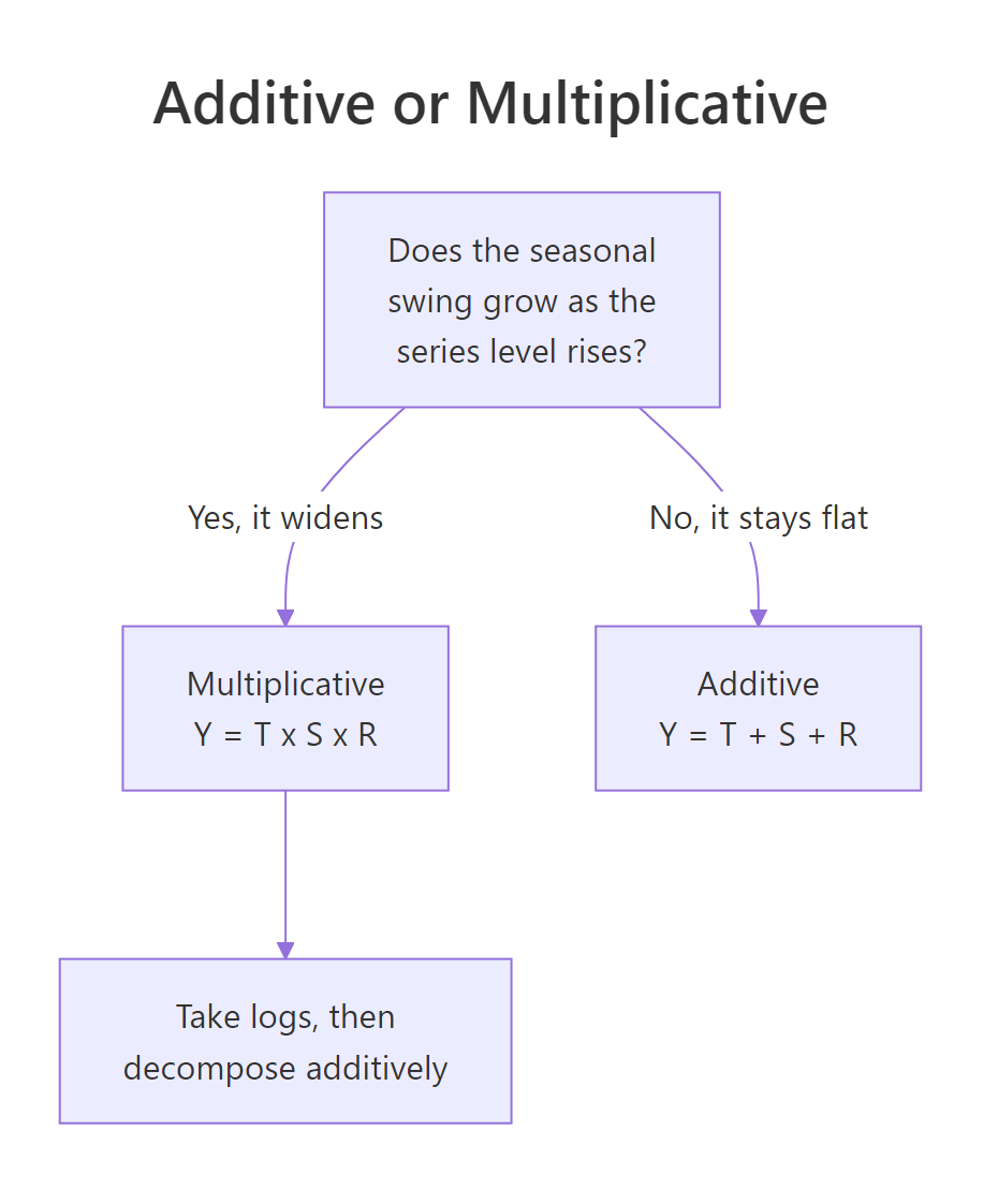
Figure 2: Choosing an additive or multiplicative model.
You do not have to guess. Measure the seasonal swing directly by taking, for each year, the gap between its highest and lowest month. If that gap grows over time, the series is multiplicative. Three short lines do it: rep(1949:1960, each = 12) builds a year label for each of the 144 months, split() uses those labels to cut the series into twelve one-year chunks, and sapply() runs max(x) - min(x) on each chunk.
The evidence is decisive. The distance between the busiest and quietest month of the year starts at 44 passengers in 1949 and grows to 232 by 1960, more than a fivefold increase. The seasonal wave is not a fixed height, it scales with the size of the airline. A swing that grows with the level is exactly what a multiplicative model describes, which is why we chose type = "multiplicative" from the start.
There is a neat trick for multiplicative series. Taking the logarithm turns multiplication into addition, because $\log(T_t \times S_t \times R_t) = \log T_t + \log S_t + \log R_t$. So a multiplicative series becomes a plain additive one on the log scale.
This is more than a curiosity. The stl() function you meet shortly only does additive decomposition, so the standard way to run STL on a multiplicative series is to decompose log(series) and then exponentiate the parts to return to the original scale.
AirPassengers forces a constant-height seasonal wave onto a series whose wave keeps growing, so the mismatch piles up in the remainder as a visible pattern. Always check the seasonal swing first, and if it grows with the level, go multiplicative or take logs.Try it: Repeat the yearly-swing measurement on nottem, then decide whether temperature is additive or multiplicative.
Click to reveal solution
Explanation: The yearly swing bounces between about 19 and 31 degrees with no upward march, because winters and summers are roughly the same distance apart every year regardless of the average. A constant-height swing means nottem is additive.
How does classical decomposition work in R?
The word "classical" is not decoration. This method dates to the early 20th century, and decompose() follows its original three-step recipe. Understanding the recipe demystifies the whole function and, just as usefully, exposes exactly where it is weak.
Step one estimates the trend with a centered moving average. For monthly data that means averaging a full year of values around each point, which averages the seasonal wave and the noise away and leaves the slow-moving level. Let's build that moving average by hand and prove it equals the trend decompose() gave us.
stats::filter() slides a set of weights along a series and returns the weighted average at each position, and sides = 2 tells it to centre the window on each point instead of only looking backwards. (We write stats:: because several packages define their own filter().) all.equal() then reports TRUE, so the trend panel you saw earlier is nothing more mysterious than this weighted average. The weights c(1/24, 1/12, ..., 1/12, 1/24) span 13 months. The two end months get half weight so that exactly 12 months of seasonal pattern are averaged out evenly, a construction known as a 2x12 moving average.
If you want the formula, here it is. Feel free to skip to the next block, the code above is the whole idea.
$$\hat{T}_t = \frac{1}{12}\left(\tfrac{1}{2}y_{t-6} + y_{t-5} + \cdots + y_{t+5} + \tfrac{1}{2}y_{t+6}\right)$$
Where $\hat{T}_t$ is the estimated trend at month $t$ and $y_{t\pm k}$ are the surrounding observations. Because the window reaches six months forward and back, there is no way to compute it for the first six or last six months. That is the source of those NA values.
Twelve values in all. On a 12-year series that is a small price, but on a three-year series it would cost you a third of the trend, including the most recent months you probably care about most.
Step two of the recipe then detrends the series (dividing it by the trend, for a multiplicative model), and step three averages those detrended values by calendar month to get the seasonal factors. Because it averages across all years, classical decomposition produces one seasonal shape and reuses it for every cycle. Those 12 factors live in components$figure. The components$seasonal slot below holds the same numbers repeated across every month of the series. To check that, we pull out two single months with window(), which slices a time series by calendar position, so c(1950, 1) means January 1950.
identical() returns TRUE: the January factor in 1950 is exactly the same number as the one in 1958. For a stable series that is fine. For one whose seasonal behavior evolves, it is too rigid.
Try it: Run a classical decomposition on the additive nottem series and plot the result.
Click to reveal solution
Explanation: Temperature has a strong, constant-height seasonal wave and no real trend, so the additive model fits well and the remainder panel looks like flat noise.
How does STL decomposition work, and why is it more flexible?
STL stands for Seasonal and Trend decomposition using Loess. Loess is a smoothing method that fits many tiny local regressions across the data instead of one rigid global average. Swapping the moving average for Loess buys three things: the seasonal shape is allowed to drift over time, the trend reaches all the way to the edges, and an optional robust mode down-weights outliers.
STL is additive only, so for the multiplicative airline series we run it on the log scale. The key argument is s.window, which controls how the seasonal component is allowed to change. Setting it to "periodic" forces a fixed seasonal shape, the same assumption classical decomposition makes.
stl() returns the three components as columns in a matrix called time.series. Notice these are log-scale numbers (the trend sits near 4.83, which is log of about 125), and notice there are no NA values. STL estimates the trend for January 1949 where classical decomposition could not, because Loess can fit near the boundary. That alone is a meaningful upgrade.
The real difference shows up when seasonality evolves. Replace "periodic" with an odd number and s.window becomes the number of years STL looks at when learning the seasonal shape, letting it change gradually. The UKgas dataset (quarterly UK gas consumption from 1960 to 1986) is perfect here, because central heating spread over those decades and the winter peak grew.
The winter (first-quarter) seasonal factor nearly doubles, from 0.316 to 0.594 on the log scale. Converted back, that is roughly a 37 percent winter bump in 1960 growing to an 81 percent bump by 1986. Classical decomposition, and STL with s.window = "periodic", would have averaged those two eras into one wrong number and hidden a real story about how Britain heats its homes.
robust = TRUE to stl() down-weights unusual observations so a one-off spike does not distort the trend and seasonal estimates. It is the STL equivalent of using a median instead of a mean, and it is cheap insurance for messy real-world data.Try it: Run STL on the co2 dataset (monthly atmospheric readings) with a periodic season, then look at the first few trend values.
Click to reveal solution
Explanation: co2 is already additive, so no log is needed. STL returns a smooth trend that climbs from about 315 parts per million, and crucially it gives a value for January 1959, the very first month, with no NA gap.
STL vs classical: which decomposition should you choose?
You now know both engines, so the choice comes down to a few honest trade-offs. Classical decomposition is fast, simple, and the textbook baseline everyone recognizes. STL is more flexible and more robust, at the cost of a couple of tuning knobs. Here is the head-to-head.
| Question | Classical decompose() |
STL stl() |
|---|---|---|
| Seasonal shape | Frozen, identical every cycle | Can change slowly over time |
| Trend at the edges | Lost (NA at both ends) | Estimated everywhere |
| Outliers | Sensitive | Optional robust mode |
| Multiplicative data | Built in via type = |
Log-transform first |
| Seasonal period | Monthly or quarterly | Any period you set |
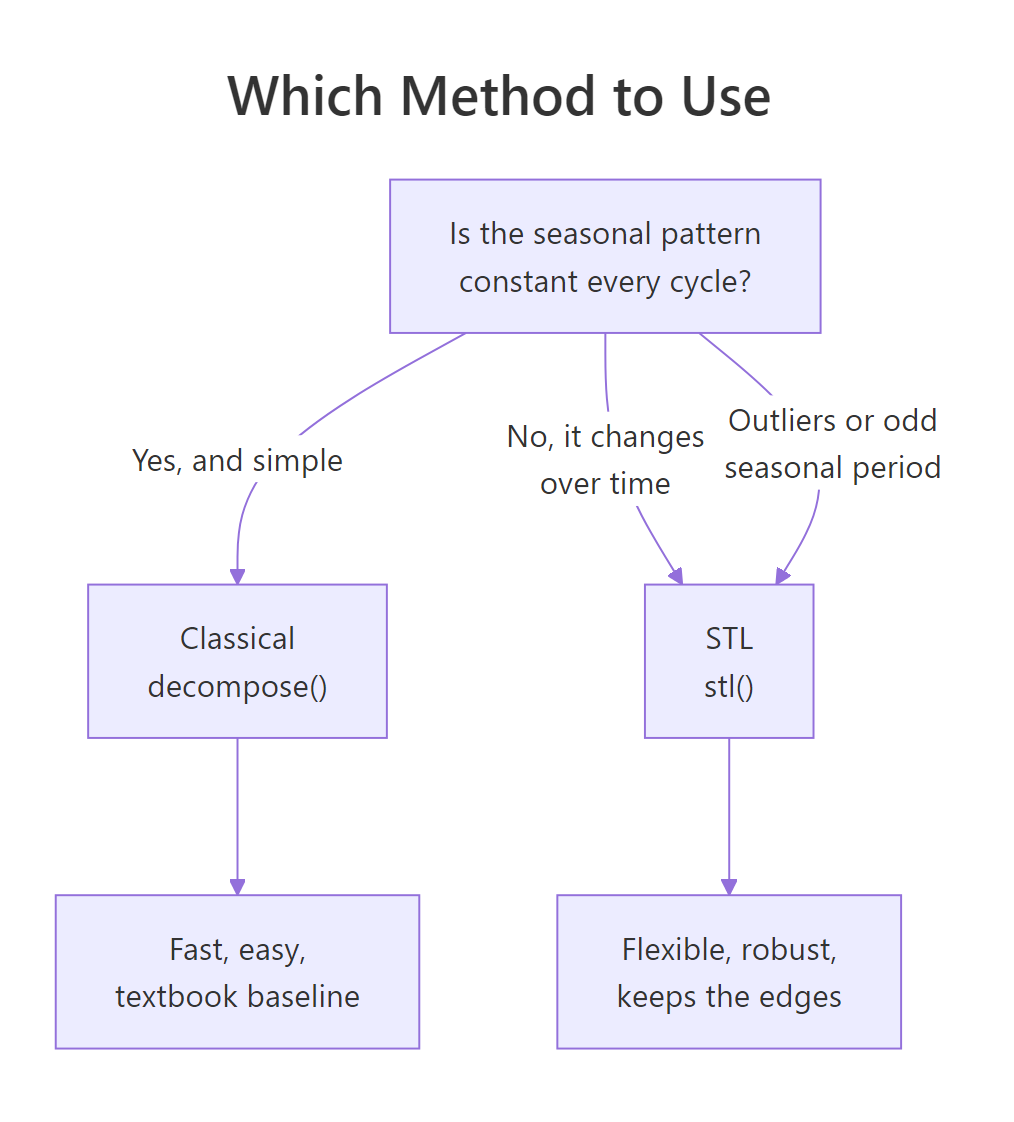
Figure 3: Deciding between classical decompose() and stl().
Whichever engine you pick, the single most common reason to decompose at all is seasonal adjustment: removing the seasonal component so the underlying signal is visible. When the news reports "seasonally adjusted unemployment," this is the operation behind it. With classical components it is one division, because the airline model is multiplicative.
Dividing out the seasonal factors leaves the trend and remainder combined, so the July spike and November dip flatten away and month-to-month changes become comparable. The STL version is the same idea, but its components are on the log scale, so we add the trend and remainder and then exponentiate.
The two adjusted series agree closely, within a passenger or two, because the airline's seasonality is stable enough that both engines see the same wave. That agreement is itself informative: when classical and STL disagree, it usually means the seasonal shape is shifting and STL is the one to trust.
Try it: The STL trend of AirPassengers is on the log scale. Exponentiate it to read the underlying passenger level in plain numbers.
Click to reveal solution
Explanation: exp() undoes the earlier log(), returning the trend to its original units. The underlying level starts around 125 passengers and rises smoothly, with the summer spikes and noise already stripped out.
Complete Example: Decompose the Mauna Loa CO2 record
Let's tie every step together on a fresh series, and deliberately pick one where classical decomposition is the right call. The co2 dataset holds monthly atmospheric carbon dioxide measured at Mauna Loa from 1959 to 1997. It has a powerful upward trend and a gentle, unchanging annual cycle, the textbook case for an additive model.
The seasonal swing here is only a few parts per million and does not grow as the level climbs from 315 into the 360s, so it is a constant height. That is additive, and it is stable, so classical decomposition will do the job well. We run it and read the trend rise directly.
The trend climbed 47.9 parts per million across the record, the real signal underneath the annual wiggle. Now the seasonal figure, which tells us the shape of that yearly cycle in absolute units.
CO2 peaks in May (+3.00) and bottoms out in October (-3.25), tracking the Northern Hemisphere growing season as plants pull carbon from the air in summer and release it in autumn. Because this is additive, seasonal adjustment is a subtraction.
With the yearly cycle removed, the adjusted values sit almost flat near 315 in early 1959 and then rise steadily, exposing the clean upward march. Finally, does STL do any better here? We compare how much variation each method leaves in the remainder, where smaller means a tighter fit.
The remainders are almost identical, 0.265 versus 0.260. When the seasonal shape genuinely is constant, STL's flexibility buys you nothing, and the simpler classical method is the sensible choice. STL earns its keep on the harder cases (shifting seasonality, outliers, or values right at the edges), not on well-behaved series like this one.
forecast and the tidyverts stack (fable and feasts) offer mstl() for multiple seasonal periods and helpers such as seasadj(), but they all rest on the trend, seasonal, and remainder logic you just built by hand.Practice Exercises
Time to combine the pieces. Each exercise uses distinct variable names so it will not clobber the tutorial's objects. Try it yourself before opening the solution.
Exercise 1: Find the warmest and coldest months
Decompose the additive nottem temperature series and use its seasonal figure to report the warmest and coldest calendar months, with their seasonal values.
Click to reveal solution
Explanation: July runs about 13 degrees above the annual mean and February about 10 below it. Because the model is additive, these are absolute temperature offsets, not percentages.
Exercise 2: Prove the parts rebuild the whole
Confirm that the multiplicative components of AirPassengers multiply back to the original series. Rebuild trend times seasonal times remainder, and check equality on the months that have a trend estimate (skip the NA edges).
Click to reveal solution
Explanation: For a multiplicative model, trend times seasonal times remainder reproduces the observed value exactly wherever the trend exists. Decomposition rearranges the data without losing any of it.
Exercise 3: Seasonally adjust UK gas demand
Use STL on the log of UKgas to seasonally adjust the quarterly gas series, then compare the average of each quarter before and after adjustment. Does winter (Q1) still dominate once the seasonal cycle is removed?
Click to reveal solution
Explanation: Raw winter (Q1) demand of 501 far exceeds summer (Q3) demand of 167. After seasonal adjustment the four quarters sit close together (325, 297, 288, 346), because the seasonal cycle, not any underlying quarter effect, was driving the gap. That flattening is exactly what seasonal adjustment is for.
Summary
Decomposition turns one hard-to-read line into three parts you can reason about, and the whole toolkit fits in a single picture.
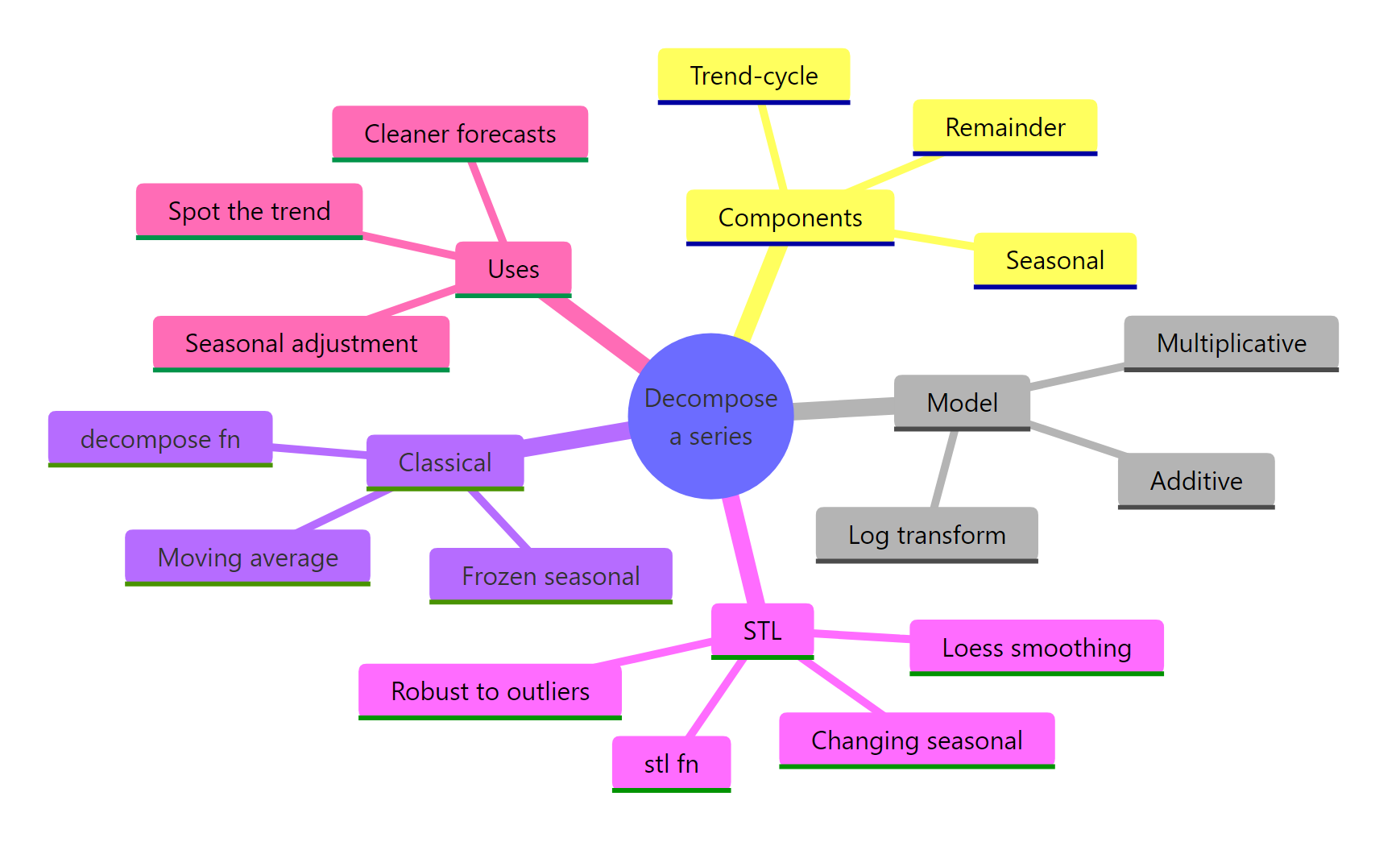
Figure 4: The whole decomposition toolkit at a glance.
| Idea | What to remember |
|---|---|
| Three components | Every series splits into trend-cycle, seasonal, and remainder |
| Additive vs multiplicative | Constant swing is additive; a swing that grows with the level is multiplicative (take logs) |
Classical decompose() |
Moving-average trend, frozen seasonal shape, NA at the edges, fast and simple |
STL stl() |
Loess-based, seasonal shape can change, no edge gaps, optional robust mode |
s.window |
"periodic" freezes the season; an odd number lets it drift over that many cycles |
| Seasonal adjustment | Remove the seasonal part to expose the real trend, the top reason to decompose |
| Choosing | Stable, simple series go classical; shifting seasonality, outliers, or edge sensitivity go STL |
Start with a plot, decide additive or multiplicative from the seasonal swing, then pick the engine that matches how stable your seasonality really is. From here, decomposition feeds directly into forecasting, because cleaner components make cleaner predictions.
Frequently Asked Questions
What is the difference between STL and classical decomposition?
Classical decompose() estimates the trend with a centered moving average and then reuses one fixed seasonal shape for every cycle. STL fits the trend and seasonal parts with Loess (many small local regressions), so the seasonal shape can change over time, the trend reaches the edges of the series with no gaps, and an optional robust mode down-weights outliers. Classical is the simpler baseline; STL is the flexible workhorse.
How do I decide between an additive and a multiplicative model?
Look at whether the seasonal swing grows as the series climbs. If the gap between the yearly high and low stays about the same size, the series is additive. If that gap widens as the level rises, like airline traffic, the series is multiplicative, so pass type = "multiplicative" to decompose() or work on the log() scale for STL.
Why does decompose() return NA values at the start and end?
The classical trend is a centered moving average that needs half a season of data on each side. For monthly data that is six months, so the first six and last six trend values cannot be computed and come back as NA. STL does not have this gap because Loess can fit right up to the boundaries.
Why do I get "time series has no or less than 2 periods"?
This is the most common first error, and it is about the input, not the method. Both functions need a ts object whose frequency is greater than 1, plus at least two full cycles of data. A plain numeric vector, or a series built with ts(x) and no frequency argument, has a frequency of 1, so there is no season to estimate and decompose() stops with that message (stl() says "series is not periodic or has less than two periods"). Rebuild the series with the right cycle length, for example ts(x, frequency = 12) for monthly data, and give it at least 24 monthly values.
Can STL handle multiplicative seasonality?
Not directly, because stl() only does additive decomposition. The standard workaround is to decompose log(series), which turns the multiplication into addition, then exponentiate the components with exp() to return to the original scale.
What does the s.window argument control?
s.window sets how quickly the seasonal shape is allowed to change. Setting it to "periodic" freezes the shape so every cycle is identical, matching the classical assumption. Setting it to an odd number lets the seasonal pattern drift, using that many cycles of context to learn the shape at each point.
References
- Hyndman, R.J. & Athanasopoulos, G. Forecasting: Principles and Practice, 3rd ed. Chapter 3: Time series decomposition. Link - the standard reference on the moving-average trend and seasonal adjustment, with the tidyverts syntax if you move beyond base R.
- Hyndman, R.J. & Athanasopoulos, G. Forecasting: Principles and Practice, 3rd ed. Section 3.6: STL decomposition. Link - read this for practical advice on choosing
s.windowandt.window. - Cleveland, R.B., Cleveland, W.S., McRae, J.E. & Terpenning, I. STL: A Seasonal-Trend Decomposition Procedure Based on Loess. Journal of Official Statistics, 6(1), 3-73 (1990). Link - the original STL paper, for exactly how the inner and outer Loess loops work.
- R Core Team.
stl(): Seasonal Decomposition of Time Series by Loess (stats package reference). Link - the full argument list, includingrobustand the window and degree settings we did not tune here. - R Core Team.
decompose(): Classical Seasonal Decomposition by Moving Averages. Link - short and worth reading once, because it states the three-step recipe in the same order we built it. - NIST/SEMATECH. e-Handbook of Statistical Methods, Section 6.4.1: Introduction to time series decomposition. Link - a compact second explanation of additive versus multiplicative if the first one did not land.
Continue Learning
- Moving Averages in R: the smoothing idea at the heart of classical decomposition, explained step by step.
- Time Series Objects in R: how to build and index the
tsobjects that decomposition depends on. - ACF and PACF in R: read the autocorrelation left in a remainder to check your decomposition captured the structure.