ARIMA in R: What AR, I, and MA Mean and How to Fit One
ARIMA is a forecasting model that combines three simple ideas: it learns from a series' own recent values (the AR part), it removes trends by working with changes instead of raw levels (the I part), and it learns from its own recent forecast errors (the MA part). You write it as ARIMA(p, d, q), and in R you fit one with Arima() or auto.arima() from the forecast package.
What is an ARIMA model, and what do p, d, and q mean?
The fastest way to see what ARIMA does is to point it at a real series and let it work. The built-in WWWusage series counts internet users connected to a server, once a minute, for 100 minutes. Let's load the forecast package and ask it to find a model on its own.
In one line, R chose a model and called it ARIMA(1,1,1). That label is the whole game: the three numbers are p, d, and q. By the end of this tutorial you will be able to read that label, understand why each number was chosen, and fit and trust a model like it yourself.
Here is what each of the three numbers controls. Keep this table nearby; every section below unpacks one row of it.
| Letter | Name | Order | What it captures |
|---|---|---|---|
| AR | Autoregressive | p | How many past values the model leans on |
| I | Integrated | d | How many times we difference to remove the trend |
| MA | Moving average | q | How many past forecast errors the model leans on |
So ARIMA(1,1,1) means: use 1 past value, difference the series once, and use 1 past error. The diagram below shows how the three pieces feed one model that then produces forecasts.
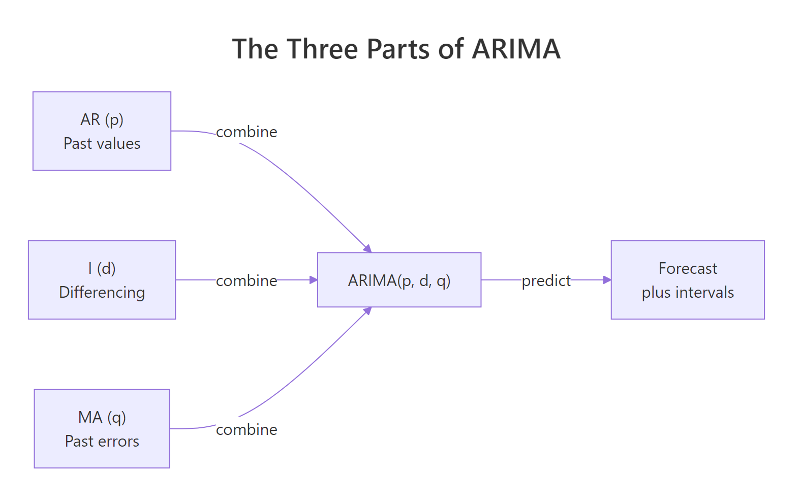
Figure 1: The three parts of ARIMA combine into one ARIMA(p, d, q) model that produces forecasts.
Before we take it apart, let's glance at the raw numbers so you can picture the data behind that model.
The counts drift upward and downward over time rather than bouncing around a fixed level. That drift is exactly what the d part exists to handle, and it is why R chose d = 1 above.
Try it: Fit an automatic model to the built-in lh series (a set of hormone measurements) and read off its (p, d, q).
Click to reveal solution
Explanation: For lh, R picks ARIMA(1,0,0), which is a pure autoregressive model of order 1. The d = 0 tells you this series did not need differencing, and q = 0 tells you no error terms were used.
What does the AR (autoregressive) part do?
The "autoregressive" idea is the most intuitive of the three: tomorrow tends to look like today. A busy web server this minute is probably busy the next minute too. AR captures that inertia by predicting each value from the value or values just before it.
An AR model of order 1, written AR(1), predicts today from yesterday using a single coefficient. In equation form it looks like this.
$$y_t = c + \phi\, y_{t-1} + \varepsilon_t$$
Where:
- $y_t$ = the value at time $t$ (what we want to predict)
- $c$ = a constant baseline
- $\phi$ = the AR coefficient, how strongly the last value pulls on this one
- $y_{t-1}$ = the previous value
- $\varepsilon_t$ = a random shock we cannot predict
A $\phi$ near 1 means strong memory (values change slowly), while a $\phi$ near 0 means almost no memory. Let's see this by building a series with a known coefficient of 0.8 and asking R to recover it. The arima.sim() function generates data from a model we specify, and Arima() fits a model back to that data.
We built the data with $\phi = 0.8$, and R estimated ar1 = 0.7765, close to the truth. The small gap is sampling noise from having only 200 points. The order = c(1, 0, 0) argument is c(p, d, q), so it says "fit one AR term, no differencing, no MA term."
Plotting the series makes the inertia visible: values wander in slow runs rather than jumping around.
That estimated coefficient of about 0.78 is the practical takeaway of the AR part. It says roughly 78 percent of a value's deviation from the mean carries over to the next step, which is why the line moves in smooth stretches.
Try it: Simulate 300 points of an AR(1) with a coefficient of 0.5, then fit an AR(1) and check that the estimate lands near 0.5.
Click to reveal solution
Explanation: The estimate ar1 = 0.5941 sits near the true 0.5, off by a bit because of random noise in the sample.
What does the MA (moving average) part do?
The MA part is the least intuitive name in all of ARIMA, so let's be precise. The moving average here has nothing to do with smoothing a series by averaging nearby points. Instead, it means the model corrects itself using its own recent forecast errors.
Picture forecasting the weather. If you predicted 20 degrees and it came in at 25, you were 5 degrees too low, and a smart forecaster nudges tomorrow's prediction up a little because of that miss. That "learn from the last surprise" behavior is exactly what an MA term does.
An MA model of order 1, written MA(1), adjusts today's value using the previous shock.
$$y_t = c + \varepsilon_t + \theta\, \varepsilon_{t-1}$$
Where:
- $\varepsilon_t$ = the current random shock
- $\theta$ = the MA coefficient, how much the last shock feeds into today
- $\varepsilon_{t-1}$ = the previous shock (the error we just made)
Let's simulate an MA(1) with a known coefficient of 0.7 and recover it, the same way we did for AR.
Here order = c(0, 0, 1) means no AR term, no differencing, one MA term. R estimated ma1 = 0.7073, right next to the 0.7 we used to build the data. The value tells us how strongly the previous minute's surprise shapes this minute's value.
Try it: Simulate an MA(1) with a coefficient of -0.6 and recover it. Negative coefficients are common and perfectly valid.
Click to reveal solution
Explanation: The estimate ma1 = -0.7011 recovers the negative sign and a magnitude close to 0.6, again with a little sampling wobble.
What does the I (integrated) part do, and when should you difference?
Both the AR and MA parts assume the series is stationary, which means its behavior does not change over time: a roughly constant average level, a roughly constant amount of wobble, and no trend heading steadily up or down. A series with a clear trend breaks that assumption, and this is the problem the I part solves.
The fix is differencing: instead of modeling the raw values, we model the change from one step to the next. If levels keep climbing, the changes usually hover around a stable level, which is stationary again.
$$y'_t = y_t - y_{t-1}$$
The d in ARIMA(p, d, q) is simply how many times we apply this. Most series need d = 0 or d = 1, and only rarely d = 2.
To see differencing rescue a trending series, look at a random walk, which is the textbook non-stationary series. We can test for stationarity with the Augmented Dickey-Fuller test from the tseries package. Its null hypothesis is "non-stationary," so a small p-value (below 0.05) is evidence that the series IS stationary.
The p-value of 0.2357 is well above 0.05, so we cannot call the raw random walk stationary. Now watch what one round of differencing does. The diff() function turns levels into step-to-step changes.
The p-value drops to 0.01, so the differenced series passes the test. That single difference is what d = 1 means in practice. R even notes the true p-value is smaller than the 0.01 it prints, which is a good sign.
Now back to real data. The WWWusage series trends, so the same test should flag it as non-stationary.
The p-value of 0.3107 confirms it is non-stationary, matching the drift we saw in the raw counts earlier. Rather than eyeball tests, you can let the forecast package pick the differencing order for you with ndiffs(), which runs a stationarity test repeatedly.
It returns 1, which is exactly the d that auto.arima() chose at the top of this tutorial. If you want a deeper treatment of these tests, see the dedicated guide on testing stationarity in R.
Try it: Use ndiffs() to find how many (non-seasonal) differences the AirPassengers series needs.
Click to reveal solution
Explanation: AirPassengers also needs one ordinary difference to remove its upward trend. It has seasonality on top of that, which we handle separately later with seasonal differencing.
How do you read ACF and PACF to choose p and q?
Once a series is stationary, two plots tell you how many AR and MA terms it likely needs. They are the autocorrelation function (ACF) and the partial autocorrelation function (PACF), and you can think of them as fingerprints of the model behind the data. If these are new to you, the ACF and PACF guide covers them in depth; here we focus on the reading rules for ARIMA.
The ACF measures how correlated the series is with itself at each lag (1 step back, 2 steps back, and so on). The PACF measures the same thing but strips out the influence of the shorter lags in between. The reading rules are short and worth memorizing.
| Pattern in the plots | Suggests |
|---|---|
| PACF cuts off sharply after lag p, ACF fades gradually | AR(p) |
| ACF cuts off sharply after lag q, PACF fades gradually | MA(q) |
| Both fade gradually | A mix of AR and MA |
Let's confirm the rules on the pure series we simulated earlier. For our AR(1) series, the PACF should show one clear spike at lag 1 and then almost nothing.
One big value (0.776) at lag 1, then a drop to near zero, is the AR(1) signature: the PACF cuts off after lag 1, so p is 1. Now the MA(1) series, whose ACF should spike once and then cut off.
The first value (1.000) is always the correlation of the series with itself at lag 0, so ignore it. The next value (0.507) is the lag-1 spike, and everything after is near zero. That cut-off after lag 1 is the MA(1) fingerprint, so q is 1.
For a real series you look at both plots together on the DIFFERENCED data, since that is what the AR and MA parts see. The ggtsdisplay() helper shows the series together with its ACF and PACF in one shot.
The diagram below sums up the decision.
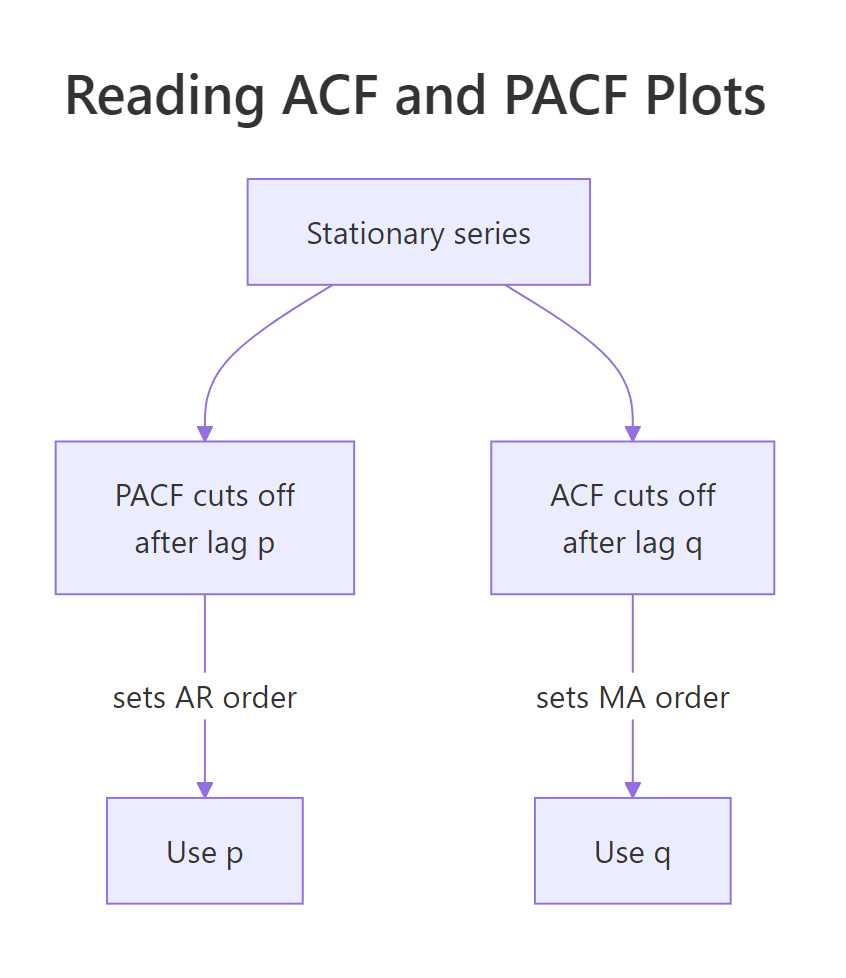
Figure 2: The PACF suggests the AR order p; the ACF suggests the MA order q.
Try it: Simulate an AR(2) series and look at its PACF. How many spikes stick out before it fades?
Click to reveal solution
Explanation: The first two values (0.684 and 0.222) stand out, then the rest fade toward zero. Two meaningful PACF spikes point to an AR order of 2, which matches how we built the series.
How do you fit an ARIMA model with Arima() and auto.arima()?
You now know what p, d, and q mean and how to guess them. Time to fit real models two ways: by hand when you want control, and automatically when you want speed.
To fit a specific model, pass the order you want to Arima(). Let's fit the ARIMA(1,1,1) we saw at the start and read its output.
The coefficients are the AR and MA weights, and the numbers to compare across models are the information criteria near the bottom. AICc (a small-sample-corrected version of AIC) balances fit against complexity, and lower is better. Let's line up three candidate orders and compare their AICc.
Among these three, ARIMA(1,1,1) has the lowest AICc (514.55), so it is the best of the bunch. Trying orders by hand is fine for a few candidates, but it does not scale. That is what auto.arima() is for: it searches many orders and returns the best by AICc.
Arima() handles a constant or drift term more gracefully and works cleanly with the rest of the forecast tools you will use for checking and plotting.The default auto.arima() uses a fast stepwise search. For a final model it is worth running the fuller search by turning off the shortcuts with stepwise = FALSE and approximation = FALSE.
The thorough search landed on ARIMA(3,1,0), a different model from the quick ARIMA(1,1,1) we started with. Its AICc of 512.42 beats that model's 514.55, which is why the deeper search preferred it. This is the workhorse of the whole toolkit: auto.arima() handles the differencing test and the order search, then fits the model, all in one call.
Try it: Fit ARIMA(2,1,2) to WWWusage and read its AICc. Is it below the 512.42 that ARIMA(3,1,0) scored?
Click to reveal solution
Explanation: ARIMA(2,1,2) scores 518.01, which is higher (worse) than the 512.42 of ARIMA(3,1,0). More terms did not help here, which is exactly why AICc penalizes needless complexity.
How do you check the model and make forecasts?
A model is only worth forecasting from if it has squeezed out all the structure it can, leaving behind residuals (the leftover errors) that look like pure random noise. If a pattern remains in the residuals, the model missed something. The checkresiduals() function runs the key test and draws the diagnostic plots.
The printout is a Ljung-Box test, whose null hypothesis is "the residuals are just noise." Here we WANT a large p-value, because a large value means we cannot find leftover structure. At 0.7218 the residuals look like white noise, so the model is trustworthy. The plots it draws, a residual time series next to its ACF and a histogram, should show no obvious patterns.
With the model validated, forecasting is one call. The forecast() function projects ahead by the number of steps you pass to h, and it returns both point forecasts and prediction intervals.
Each row is one future minute. The Point Forecast is the single best guess, and the four interval columns give ranges: the model is 80 percent sure the value lands between the Lo 80 and Hi 80 columns, and 95 percent sure between Lo 95 and Hi 95. Notice the intervals widen further out, because uncertainty compounds the further ahead you look. A picture makes that fan of uncertainty obvious.
Try it: Forecast WWWusage five periods ahead from best_fit and read the first point forecast.
Click to reveal solution
Explanation: The first row is period 101 with a point forecast of about 219.66, and its 95 percent interval runs from roughly 213.6 to 225.8.
How do you model seasonal data with seasonal ARIMA?
Many real series repeat on a calendar: retail sales peak every December, airline traffic swells every summer. ARIMA handles this with a seasonal extension, often called SARIMA, that adds a second set of terms operating at the seasonal lag. The full notation is ARIMA(p, d, q)(P, D, Q)[m], where the second bracket is the seasonal AR, differencing, and MA orders, and m is the number of periods in one cycle (12 for monthly data).
The good news is that auto.arima() handles all of this for you when the series carries a frequency. The classic AirPassengers series records monthly airline passengers and has strong yearly seasonality.
Read the label in two halves. The non-seasonal part (2,1,1) works step-to-step (here month-to-month), and the seasonal part (0,1,0)[12] says: take one seasonal difference at lag 12, comparing each month to the same month last year, with no seasonal AR or MA terms. That single seasonal difference is what strips out the repeating yearly pattern.
Forecasting works exactly as before, and the plot shows the seasonal shape continuing into the future.
Try it: Use nsdiffs() to find how many SEASONAL differences AirPassengers needs.
Click to reveal solution
Explanation: nsdiffs() returns 1, which matches the seasonal D = 1 that auto.arima() chose. It measures seasonal (year-over-year) differencing, while ndiffs() measures the ordinary kind.
Complete Example: Forecasting the Nile end to end
Let's put every step together on a fresh series. The built-in Nile series records the annual flow of the river from 1871 to 1970. We will plot the series, make it stationary, fit and check a model, then forecast, reusing the full workflow you will apply to any series.
First, plot the raw data to get a feel for it.
Next, ask how many differences it needs, then let auto.arima() build the model.
R chose ARIMA(1,1,1): one difference, one AR term, one MA term. Before trusting it, check the residuals.
The Ljung-Box p-value of 0.2863 is comfortably above 0.05, so the residuals pass as noise. Now forecast the next ten years and plot the result.
The point forecasts settle near 842, which is sensible for a differenced series with no trend: once past the last observations, the best guess is a stable level, and the honest widening of the intervals shows how uncertainty grows over a ten-year horizon.
Frequently Asked Questions
What is the difference between ARIMA and ARMA? ARMA models a stationary series directly with AR and MA terms. ARIMA adds the "I" step, differencing the series first so that trending, non-stationary data becomes stationary. In R, ARIMA(p, 0, q) is just an ARMA(p, q).
Should I use auto.arima() or choose the order myself? Start with auto.arima(); it is fast and reliable. Choose orders yourself when you have domain knowledge to test a specific structure, or when you want to compare a handful of candidates by AICc. Always validate whichever you pick with residual checks.
What is a good AIC or AICc value? There is no universal threshold; these numbers only mean something in comparison. Fit several models to the same series and prefer the one with the lowest AICc. Comparing AICc across different series is meaningless.
My residuals fail the Ljung-Box test. What now? A small p-value means leftover structure. Try adding an AR or MA term, check whether you need another difference, and for calendar data confirm you captured the seasonality. Re-run checkresiduals() until the p-value clears 0.05.
Can ARIMA use other predictors like promotions or weather? Yes. Pass extra regressors to the xreg argument of Arima() or auto.arima() to fit a regression model with ARIMA errors, sometimes called ARIMAX.
Practice Exercises
These combine several ideas from the tutorial. Each starter block runs as-is so you can experiment; write your solution, then reveal ours to compare. The exercises use their own variable names so they will not clash with the code above.
Exercise 1: Manual versus automatic on lh
Fit the lh series two ways, as a manual ARIMA(1,0,0) and with a thorough auto.arima(), then compare their AICc values. Which model does the search prefer, and by how much?
Click to reveal solution
Explanation: The manual AR(1) scores 65.30, but the thorough search finds a better model at 63.99. That better model is an ARIMA(0,0,2), a pure MA(2), which fits lh slightly better than the AR(1) does.
Exercise 2: Read a forecast interval
Forecast the lh series eight periods ahead with auto.arima(), then report the 95 percent prediction interval (the Lo 95 and Hi 95 columns) of the FIRST forecast row.
Click to reveal solution
Explanation: The first row (period 49) has a point forecast near 2.69, with a 95 percent interval running from about 1.80 to 3.58. The interval widens in later rows as uncertainty grows.
Exercise 3: A seasonal model from scratch
Fit a seasonal ARIMA to the monthly USAccDeaths series (accidental deaths in the US) with auto.arima(), identify its seasonal (P, D, Q)[12] part, then forecast the next 12 months.
Click to reveal solution
Explanation: The model is ARIMA(0,1,1)(0,1,1)[12]. The seasonal part (0,1,1)[12] takes one seasonal difference and adds one seasonal MA term (sma1), and the forecast faithfully repeats the summer peak and winter dip you would expect from accident data.
Summary
ARIMA is three plain ideas combined, and reading an ARIMA(p, d, q) label is just naming each one. The workflow below is the same every time: understand the series, make it stationary, pick and fit a model, check it, then forecast.

Figure 3: The end-to-end ARIMA modeling workflow, from plotting to forecasting.
| Step | What it does | Key function |
|---|---|---|
| AR (p) | Learns from past values | Arima(order = c(p, 0, 0)) |
| I (d) | Differences away the trend | diff(), ndiffs() |
| MA (q) | Learns from past errors | Arima(order = c(0, 0, q)) |
| Choose orders | Reads the fingerprints | ggtsdisplay(), Acf(), Pacf() |
| Fit | Estimates the model | Arima(), auto.arima() |
| Check | Confirms residuals are noise | checkresiduals() |
| Forecast | Projects ahead with intervals | forecast() |
Keep these takeaways close:
- AR uses past values, MA uses past errors, I differences away the trend. The three orders p, d, q say how many of each.
- Difference until stationary. Use
ndiffs()for the ordinary order andnsdiffs()for the seasonal one, rather than guessing. - Let auto.arima() do the search, then verify. Add
stepwise = FALSEfor the final model, and never forecast beforecheckresiduals()clears. - Seasonal ARIMA is the same idea at the seasonal lag. The (P, D, Q)[m] block handles calendar cycles automatically.
References
- Hyndman, R.J., & Athanasopoulos, G. - Forecasting: Principles and Practice, 3rd edition. Chapter 9: ARIMA models. Link
- Hyndman, R.J., & Khandakar, Y. - "Automatic Time Series Forecasting: The forecast Package for R." Journal of Statistical Software, 27(3), 2008. Link
- forecast package -
auto.arima()reference. Link - forecast package -
Arima()reference. Link - Box, G.E.P., Jenkins, G.M., Reinsel, G.C., & Ljung, G.M. - Time Series Analysis: Forecasting and Control, 5th edition. Wiley (2015).
- R Core Team - An Introduction to R, Time Series section. Link
Continue Learning
- ACF and PACF in R - go deeper on the autocorrelation plots you use to pick p and q.
- Test Stationarity in R - the full set of unit-root and stationarity tests behind differencing.
- ETS Models in R - exponential smoothing, the other major forecasting family and a natural comparison to ARIMA.