Holt-Winters in R: Additive or Multiplicative Seasonality?
Holt-Winters is a forecasting method that smooths three things at once, the level, the trend, and the repeating seasonal pattern, so it can project a series that both drifts upward and cycles every year. In R you fit it with HoltWinters(), and the one real modelling decision you make is whether the seasonal swing is additive (a fixed size) or multiplicative (a percentage of the level).
This tutorial builds Holt-Winters from the ground up. You will fit your first seasonal forecast in the first code block, then open the method up piece by piece: what the three components are, what the smoothing parameters control, and how to make the additive-versus-multiplicative call with confidence. Every code block runs in your browser, so you can change a number and re-run it as you read. We use the forecast package on top of base R, and no prior forecasting experience beyond a basic idea of a time series is assumed.
How is Holt-Winters different from simpler exponential smoothing?
A plain moving average smooths the seasonal peaks and troughs away, so it cannot project them. Simple exponential smoothing tracks the level, and Holt's method adds a trend, but neither one captures the fact that airline traffic peaks every July. Holt-Winters adds a third smoother for the season, so it can forecast the peaks and troughs, not just the middle of the series. Here is that payoff on the classic monthly airline-passenger data before we open the engine up.
We fit a Holt-Winters model to AirPassengers (monthly totals from 1949 to 1960) and ask for the next twelve months. The seasonal = "multiplicative" argument tells R the seasonal swings grow with the series, which we will justify shortly.
Walk-through. HoltWinters() looked at the 144 months of history and estimated a level, a slope, and a twelve-month seasonal shape. forecast(fit, h = 12) projected all three forward one year. The Point Forecast column is the model's best guess for each month, and the four Lo/Hi columns are the 80% and 95% prediction intervals, the range the true value should fall in most of the time.
Interpretation. Look at the shape of the point forecasts: a summer peak in July (666) and a winter dip in November (420), riding on top of a level that is higher than any year before it. That is the whole promise of Holt-Winters. It carries the trend and the seasonal rhythm into the future together. A plot makes the pattern obvious.
The dark line is the history, the blue line is the forecast, and the shaded band is the uncertainty. Notice how the forecast repeats the seasonal wave while continuing to climb.
Try it: You asked for twelve months above. Forecast only the next six months instead, and print just the point forecasts (the $mean element) rounded to one decimal.
Click to reveal solution
Explanation: The $mean element holds just the point forecasts, without the prediction-interval columns. Because you reused fit, the six months match the first six rows of the twelve-month table.
What are the three components of a seasonal time series?
Before you can smooth a season, it helps to see the pieces Holt-Winters is tracking. Any seasonal series can be split into three parts, and R can pull them apart for you so you can look at each one.
- Level: where the series sits right now, ignoring the wiggles. Think of it as the current baseline.
- Trend: the direction and speed the level is drifting, up or down, per period.
- Seasonal: the repeating within-year pattern, the same shape that comes back every twelve months.
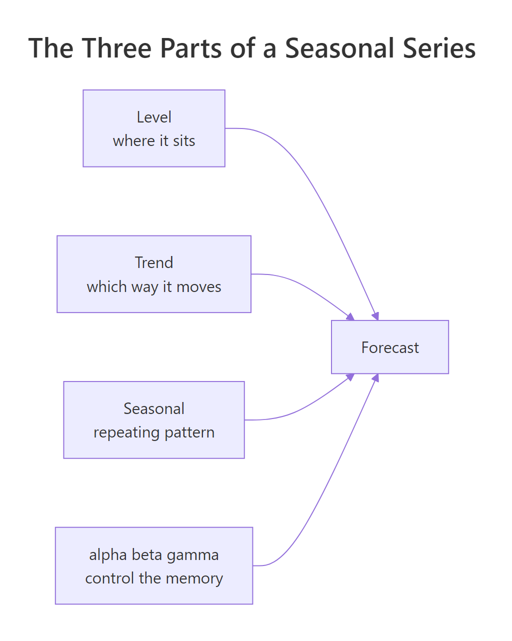
Figure 2: Holt-Winters smooths level, trend, and season separately, then combines them into a forecast.
The decompose() function estimates these parts directly. It is a quick diagnostic, separate from the forecasting model, and a good way to build intuition. Here we ask for a multiplicative split of AirPassengers and print the twelve seasonal factors.
Walk-through. comp$figure holds one number per month, January through December. In a multiplicative split these are ratios centred on 1. A value of 1.227 for July means July traffic runs about 23% above the yearly average, and 0.801 for November means November runs about 20% below it.
Interpretation. These twelve factors are the seasonal shape Holt-Winters will keep re-estimating and projecting forward. Plotting the full decomposition shows the level, trend, and seasonal parts stacked so you can read each on its own.
Try it: Run decompose() again, but ask for an additive split, and print its seasonal figure rounded to one decimal. Additive factors are measured in passengers, not ratios.
Click to reveal solution
Explanation: In an additive split the seasonal factors are absolute passenger counts that sum to about zero: July adds about 64 passengers, November subtracts about 54. Compare this to the multiplicative version above, where the same seasons were expressed as percentages of the level.
What do alpha, beta, and gamma control?
Holt-Winters has exactly three tuning knobs, named with the Greek letters alpha, beta, and gamma. Each one is a memory dial for one of the three components. A dial near 0 gives the component a long memory, so it changes slowly and leans on the whole history. A dial near 1 gives it a short memory, so it snaps to the most recent observation and forgets the past quickly.
- alpha controls the level: how fast the baseline reacts to the newest data point.
- beta controls the trend: how fast the slope updates when the series speeds up or slows down.
- gamma controls the season: how fast the seasonal shape is allowed to drift year to year.
Under the hood, every update is a weighted average between new information and the old estimate, and the dial is the weight. For the level, for example:
$$\ell_t = \alpha \cdot (\text{new information}) + (1 - \alpha)\cdot(\text{previous estimate})$$
Where:
- $\ell_t$ is the updated level at time $t$
- $\alpha$ is the level dial between 0 and 1
- new information is the latest observation, adjusted for its season
- previous estimate is last period's level projected forward by the trend
If the math is not your thing, skip it. The one idea to keep is that a bigger dial means faster reaction. You rarely set these by hand. When you leave them at their default, R finds the values that make the model's one-step-ahead errors as small as possible. Let us read the three values R chose for the airline model.
Walk-through. These three numbers were estimated automatically when you called HoltWinters() back in the first section. We pulled them off the fitted object with fit$alpha and friends, and wrapped each in unname() just to keep the printout tidy.
Interpretation. Alpha of 0.276 is a moderate level memory, so the baseline moves but does not lurch. Beta of 0.033 is very small, meaning the trend is treated as steady and barely re-estimated. Gamma of 0.871 is high, which says the seasonal shape is allowed to update quickly, letting the growing summer peaks be captured as they get bigger each year.
Try it: Fit a multiplicative Holt-Winters model to a different built-in series, UKgas (quarterly UK gas consumption), and print its three smoothing parameters the same way.
Click to reveal solution
Explanation: Gas consumption has a very stable level (alpha near 0, long memory) but a trend that updates fully each quarter (beta of 1). Different series lead R to different dial settings, which is exactly the point of letting it optimise.
Additive or multiplicative seasonality: how do you choose?
This is the decision in the title, and it is the only one that really matters. The rule is about the size of the seasonal swings as the series grows.
- If the swings stay a constant size in absolute units, year after year, use additive seasonality. The season is added on: level plus a fixed amount.
- If the swings grow with the level, so busier years have bigger peaks and deeper troughs, use multiplicative seasonality. The season is multiplied in: level times a percentage.
- If the series contains zeros or negative values, you must use additive, because multiplying by a percentage of zero makes no sense.
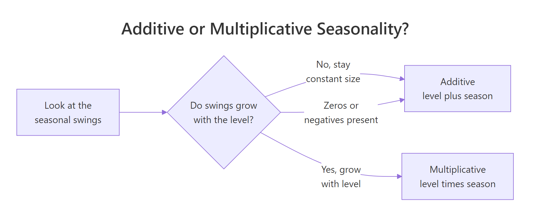
Figure 1: Pick additive when seasonal swings stay a constant size, multiplicative when they grow with the level.
The two forecast equations make the difference concrete. The additive forecast adds the seasonal term:
$$\hat{y}_{t+h} = \underbrace{\ell_t}_{\text{level}} + \underbrace{h\,b_t}_{\text{trend}} + \underbrace{s_{t+h-m}}_{\text{season}}$$
The multiplicative forecast multiplies by it:
$$\hat{y}_{t+h} = (\ell_t + h\,b_t)\times s_{t+h-m}$$
Where $\ell_t$ is the level, $b_t$ is the trend per period, $s$ is the seasonal factor, $m$ is the number of periods in a year (12 for monthly data), and $h$ is how far ahead you forecast. In the additive form the season is a number of passengers; in the multiplicative form it is a ratio like 1.23.
For AirPassengers, the summer peaks clearly get taller every year, so multiplicative should fit better. You do not have to guess. Fit both and compare their in-sample error. HoltWinters() stores the sum of squared errors in $SSE, and smaller is better.
Walk-through. We fit the same series two ways, changing only the seasonal argument, then printed both error totals side by side. The $SSE is the total squared gap between the fitted values and the actual data across all 144 months.
Interpretation. The multiplicative model's error (16571) is about 24% lower than the additive model's (21860). That matches what your eye saw in the plots: because the seasonal swings grow with the level, letting the season scale as a percentage fits the airline data much better.
Try it: You already have fit_add and fit_mul. Write one line that prints the word "additive" or "multiplicative" depending on which has the smaller SSE, so the choice is made in code rather than by eye.
Click to reveal solution
Explanation: ifelse() checks the condition and returns one of two strings. Wrapping the SSE comparison this way is a handy pattern when you loop over many series and want the seasonality type chosen automatically for each.
When is additive seasonality the right call?
Multiplicative won for airline traffic, but plenty of series are the opposite. Think of anything whose seasonal swing is a roughly fixed amount no matter how high the baseline climbs: monthly heating degree-days, a store that always sells about 300 extra units in December, or temperatures that rise and fall by the same number of degrees each year. For those, additive is both the correct and the more stable choice.
To see it cleanly, let us build a series by hand where we control the seasonality. We give it a rising level but a seasonal swing that stays the same size every year. Because we set the random seed, you will get exactly these numbers when you run it.
Walk-through. We built a 120-month series: a straight-line trend rising from about 150 to 390, plus a twelve-month swing pattern that repeats unchanged every year, plus a little random noise. The seasonal high (July, +55) and low (February, -45) are the same absolute size in year 1 and year 10, even though the level nearly triples.
Interpretation. This is additive seasonality by construction. A quick plot confirms the swings look like a constant-width band around a rising line rather than a widening funnel.
Now fit both seasonality types and compare, exactly as before.
Walk-through. Same two-way comparison, this time on the constant-swing series. The additive model's error total is far lower.
Interpretation. Additive wins by about 38% here (16108 versus 26062), the mirror image of the airline result. When the swings do not grow with the level, forcing a multiplicative season makes the model overstate the seasonality at high levels and understate it at low ones, which shows up as a larger error.
Try it: Forecast the additive model sales_add twelve months into the future and print the point forecasts rounded to whole numbers.
Click to reveal solution
Explanation: The forecast continues the rising level while adding the same fixed seasonal swing, so the 2025 July peak sits about 100 units above the February low, the same gap the series has always had.
How do you check whether the model fits well?
A low SSE says a model beat its sibling, but not that it is trustworthy. The real test is the residuals, the leftover gaps between the fitted values and the data. If Holt-Winters has captured the level, trend, and season, what remains should look like random noise with no pattern left in it. The checkresiduals() function runs that test for you.
Walk-through. checkresiduals() draws a three-panel plot (the residuals over time, their autocorrelation, and their distribution) and runs a Ljung-Box test. That test asks a single question: is there leftover autocorrelation, meaning pattern the model failed to catch? A small p-value says yes, some structure remains.
Interpretation. The p-value of 0.011 is below 0.05, so a little autocorrelation is still present. That is common and not a disaster on a series as long as this one. The residual plot has no giant systematic wave, which is what you most want to avoid. In practice you weigh this against the forecast accuracy rather than demanding a perfect white-noise result.
Try it: Numbers back up the plot. Print the full training-set accuracy table for fit using accuracy() on a one-step forecast, rounded to two decimals, and read off the RMSE and MAPE.
Click to reveal solution
Explanation: RMSE of 11.2 is the typical error in passengers, and MAPE of 3.02 means the fitted values are off by about 3% on average. MAPE is the easiest to explain to a non-technical audience because it is a plain percentage.
HoltWinters(), hw(), or ets(): which should you use?
R gives you three ways to fit a Holt-Winters model, and it helps to know when to reach for each.
| Function | Package | Best for |
|---|---|---|
HoltWinters() |
base stats |
Learning the method; direct control; no extra install |
hw() |
forecast |
Cleaner forecasts, prediction intervals, optional damped trend |
ets() |
forecast |
Automatic selection of the whole model, including seasonality type |
The standout is ets(). It searches over additive and multiplicative options for the error, the trend, and the season, then picks the combination with the best information criterion. You do not tell it the seasonality type; it decides. Let us let it choose a model for the airline data.
Walk-through. The header ETS(M,Ad,M) is the model ets() chose: Multiplicative error, Additive damped trend, and Multiplicative season. It agrees with our hand analysis that the season is multiplicative, and it went one step further by adding a damped trend (the phi = 0.98 parameter).
Interpretation. Damping means the trend is allowed to flatten out over long horizons instead of climbing forever in a straight line. That phi of 0.98 is a gentle damping. Because reckless straight-line trends are a classic way forecasts go wrong far into the future, damping is worth understanding. But it is not always an improvement, so test it rather than assume it. Here we compare an undamped and a damped multiplicative model by their corrected AIC, where lower is better.
Walk-through. We fit two hw() models that differ only by the damped flag, then compared their aicc, a score that rewards fit while penalising extra parameters.
Interpretation. Here the undamped model scores lower (1410.5 versus 1424.8), so on this series damping does not pay off. The lesson is not "damping is bad" but "check, do not assume." Damping helps most when a strong trend would otherwise run away over a long forecast horizon.
Try it: Run ets() on the UKgas series and read the three-letter model code it prints in the header. What error, trend, and season did it choose?
Click to reveal solution
Explanation: ETS(M,A,M) means multiplicative error, additive (undamped) trend, multiplicative season. Gas consumption has strong, growing seasonal swings, so a multiplicative season is the natural pick here too.
Complete Example: Forecasting Airline Passengers End to End
Let us put the whole workflow together and, crucially, test the forecast honestly. In-sample error can flatter a model, so we hold out the last two years, fit only on the earlier data, forecast the gap, and compare the forecast to what actually happened.
Walk-through. window() splits the series in time: train is 1949 to 1958, test is the final 24 months. We fit on train only, forecast 24 months, and accuracy(fc, test) scores those forecasts against the held-out truth. The Training set row is in-sample error; the Test set row is the honest out-of-sample error.
Interpretation. In-sample MAPE was a tidy 3.10%, but on genuinely unseen months it rose to 7.26%. That gap is normal and healthy to measure. The model still tracks the seasonal shape two years out, it just loses some precision, which the widening prediction interval already warned us about. A plot shows the forecast against the actual values.
The red line is what actually happened; the blue forecast stays close through 1959 and drifts a little in 1960.
Practice Exercises
Work these in order. They combine the pieces from above, so use fresh variable names to avoid overwriting the tutorial's objects.
Exercise 1: Forecast quarterly gas demand
Fit a multiplicative Holt-Winters model to the UKgas series (quarterly, so its season has four periods) and forecast the next eight quarters. Print the point forecasts rounded to one decimal.
Click to reveal solution
Explanation: Gas demand peaks hard in the winter quarter (Qtr1) and bottoms out in summer (Qtr3). Because the season is multiplicative, those peaks keep growing with the rising level, so 1988's winter forecast is higher than 1987's.
Exercise 2: Which seasonality type generalises better?
In the tutorial, multiplicative won on the full-sample airline data. Does it also win out of sample? Hold out the last two years of AirPassengers, fit both an additive and a multiplicative model on the rest, and compare their test-set RMSE and MAPE. Report which one generalises better on this split.
Click to reveal solution
Explanation: This is the honest twist. Multiplicative fit the full sample better, yet on this particular 24-month holdout the additive model edges it on both RMSE (35.79 versus 36.61) and MAPE (6.69 versus 7.26). They are very close. The takeaway is that in-sample SSE and out-of-sample accuracy can disagree, so validate on a holdout and let both the data structure and the test error inform your final choice.
Exercise 3: Beat a damped model with automatic selection
Compare two models on AirPassengers: the fully automatic ets() model and an explicitly damped multiplicative hw() model. Print both corrected AIC values and report which model R prefers and what three-letter type ets() selected.
Click to reveal solution
Explanation: The automatic ets() model scores a lower corrected AIC (1400.6 versus 1424.8), so R prefers it. It chose ETS(M,Ad,M): multiplicative error, additive damped trend, multiplicative season. Automatic selection found a strong model without you specifying anything.
Frequently Asked Questions
What is the difference between HoltWinters() and ets()?
HoltWinters() lives in base R, fits the exact model you ask for, and optimises alpha, beta and gamma for you. ets() in the forecast package goes further: it searches additive and multiplicative options for the error, trend and season, then picks the best by an information criterion, so it also makes the seasonality decision for you. Reach for HoltWinters() when you want to see and control every knob, and ets() when you want a fast, strong baseline.
Why do I get "time series has no or less than 2 periods"?
Holt-Winters estimates its starting seasonal shape from at least two complete cycles, so a monthly series needs 24 or more observations and a quarterly one needs 8. With less history than that, R stops with this error. Collect more data, or drop to a non-seasonal method such as Holt's linear trend.
Do I need to set the seasonal frequency on my data first?
Yes. HoltWinters() reads the length of the season from the frequency of your ts object. If you build the series without setting it, the frequency defaults to 1. R then has no season to estimate, so the seasonal fit fails. Set it when you create the series, for example ts(x, frequency = 12) for monthly data or frequency = 4 for quarterly.
Can Holt-Winters model two seasonal patterns at once?
No. HoltWinters() and ets() each track a single seasonal period. A series with both a weekly and a yearly cycle, such as daily electricity demand, needs a method built for multiple seasonality, such as tbats() or a regression with fourier() terms, both in the forecast package.
Is additive or multiplicative the default in HoltWinters()?
Additive. HoltWinters(x) with no seasonal argument fits an additive season, because that is the first option R falls back to. Since the choice changes the forecast, set seasonal = "multiplicative" whenever the swings grow with the level, and let ets() decide when you are unsure.
Summary
Holt-Winters extends exponential smoothing to series that both trend and cycle, by smoothing the level, the trend, and the season together. The one decision that shapes your forecast is the seasonality type, and it comes down to whether the swings grow with the level.
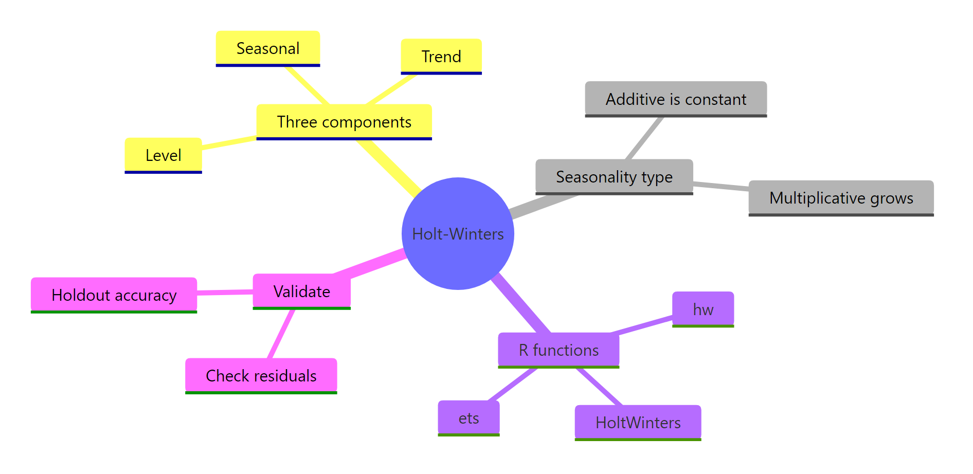
Figure 3: The Holt-Winters workflow at a glance.
| Idea | What to remember |
|---|---|
| Three components | Level, trend, and season, each smoothed separately, then combined |
| alpha, beta, gamma | Memory dials near 0 mean long memory, near 1 mean fast reaction |
| Additive season | Constant-size swings; season added as a fixed amount |
| Multiplicative season | Swings grow with the level; season multiplied as a percentage |
| Choosing the type | Compare $SSE, watch the amplitude, use additive if the data has zeros |
| Checking the fit | Residuals should look like noise; validate on a holdout, not just in-sample |
| Which function | HoltWinters() to learn, hw() for clean forecasts, ets() to auto-select |
Start with ets() for a fast, strong baseline, then reach for HoltWinters() when you want to control and inspect each component yourself.
References
- Hyndman, R.J., & Athanasopoulos, G. Forecasting: Principles and Practice, 3rd edition, Chapter 8.3: Holt-Winters' seasonal method. Link
- R Core Team.
HoltWintersfunction reference, basestatspackage. Link - Hyndman, R.J. et al.
forecastpackage documentation,hw()andets()reference. Link - Winters, P.R. (1960). Forecasting Sales by Exponentially Weighted Moving Averages. Management Science, 6(3), 324-342. Link
- Hyndman, R.J., Koehler, A.B., Ord, J.K., & Snyder, R.D. (2008). Forecasting with Exponential Smoothing: The State Space Approach. Springer. Link
- R Core Team.
decomposefunction reference, basestatspackage. Link
Continue Learning
- Exponential Smoothing in R - the level-only smoother that Holt-Winters builds on, and where the alpha parameter first appears.
- ETS Models in R - the state-space framework behind
ets()that generalises Holt-Winters and automates the additive-versus-multiplicative choice. - Time Series Decomposition in R - a closer look at splitting a series into trend, seasonal, and remainder parts.