Holt's Method in R: Forecast Trend Without Seasonality
Holt's method, also called double exponential smoothing, extends simple exponential smoothing by tracking a slope as well as a level, so its forecast climbs or falls in a straight line instead of staying flat. The holt() function in R's forecast package fits the model and tunes both smoothing dials for you.
Simple exponential smoothing (SES) is the base case: it estimates one number, the current level, and forecasts that same number forever, which is why its forecast is a flat horizontal line. That works beautifully for a series that only wobbles around a steady level, but it falls apart the moment the data trends up or down. This tutorial builds Holt's method up from that gap, one piece at a time, using the built-in airmiles series (annual airline passenger miles, no downloads needed) so you can run every line yourself. We stay in the well-tested forecast package throughout.
What does Holt's method add to simple exponential smoothing?
A trending series has somewhere to go, but SES has no way to follow it. SES tracks only a level, so its best guess about the future is "wherever the level is now," repeated forever. Holt's method adds a second moving piece: an estimate of the slope, which it carries forward. The result is a forecast that keeps rising (or falling) instead of freezing in place. Let's see it before we unpack the theory.
The block below loads the forecast package, fits Holt's method to the airmiles series, and asks for a six-year forecast.
Look at the Point Forecast column. Unlike SES, these numbers are not all the same: they climb steadily from 32,764 in 1961 to 43,299 in 1966. Each year is about 2,107 higher than the year before, a constant step that is exactly the trend Holt estimated. The four other columns are 80% and 95% prediction intervals (the plausible range around the forecast), and they widen the further out you look.
To feel how different that is from SES, fit both to the same data and compare their final-year forecasts side by side.
SES parks its forecast at 30,514 for every future year, roughly the last observed level. Holt, having estimated an upward trend, projects 43,299 by 1966. On a series that is clearly growing, that gap is the difference between a forecast that ignores the trend and one that respects it. A picture makes it obvious.
The blue line is the point forecast, sloping upward to continue the trend of the history, wrapped in shaded prediction bands that fan out with the horizon.
Try it: Ask holt() for a 3-year forecast of airmiles instead of 6, and confirm each year is higher than the last.
Click to reveal solution
Explanation: Only the horizon h changes. Each point forecast is about 2,107 higher than the one before, because Holt keeps adding the estimated trend at every step.
How do the level and trend equations work?
Holt runs two smoothing updates at every time step instead of one. The first tracks the level, just like SES. The second tracks the trend, the slope from one point to the next. Each update is a weighted blend controlled by its own dial: alpha for the level and beta for the trend.

Figure 1: Holt runs two smoothing updates each step: one for the level, one for the trend.
The level update is SES with a twist. Instead of blending the new observation with the old level, it blends the new observation with the old level plus the old trend (a one-step-ahead guess of where the level should be now). Writing the level at time $t$ as $\ell_t$ and the trend as $b_t$:
$$\ell_t = \alpha\, y_t + (1 - \alpha)\,(\ell_{t-1} + b_{t-1})$$
The trend update then blends the newest observed slope (how much the level just changed) with the previous trend estimate:
$$b_t = \beta\,(\ell_t - \ell_{t-1}) + (1 - \beta)\,b_{t-1}$$
And the forecast for any future step is the latest level plus that many steps of the latest trend:
$$\hat{y}_{t+h\,|\,t} = \ell_t + h\, b_t$$
Where:
- $\ell_t$ = the level, the smoothed value at time $t$
- $b_t$ = the trend, the smoothed slope at time $t$
- $\alpha$ = the level dial, between 0 and 1
- $\beta$ = the trend dial, between 0 and 1
- $h$ = how many steps ahead you are forecasting
The clearest way to feel this is to run both updates by hand on a tiny series. Below we smooth six numbers, starting the level at the first value and the trend at the first change (the second value minus the first).
Walk through the third step to see the two updates in action. The level guess before seeing y[3] = 8 is the old level plus the old trend, 7 + 2 = 9; blending that with the new 8 gives 0.5 * 8 + 0.5 * 9 = 8.5, the third level. The observed slope is 8.5 - 7 = 1.5, and blending that with the old trend of 2 gives 0.3 * 1.5 + 0.7 * 2 = 1.85, the third trend. Both estimates move a little toward the fresh data and a lot toward their own history, which is what smoothing means.
Now use those final numbers to forecast. The last level is 14.583 and the last trend is 1.979, so each future step just adds another 1.979.
There is the forecast equation made concrete: 14.583 plus one trend is 16.562, plus two trends is 18.541, plus three is 20.521. The point forecast is nothing more than the final level extended by the final slope.
Try it: Smooth the same y vector but with a gentler trend dial of beta = 0.1, and watch the trend estimates settle more smoothly.
Click to reveal solution
Explanation: With beta = 0.1 the trend leans 90% on its own past, so it barely reacts to each new observed slope and stays close to its starting value of 2. A small beta gives a steady, slowly changing trend.
How does holt() estimate alpha and beta?
You do not have to guess alpha and beta. By default, holt() finds the pair of values (along with the starting level and trend) that make the model fit the historical data as closely as possible. It measures fit with the sum of squared errors, the total of the squared gaps between each actual value and the model's one-step-ahead forecast of it. There is no tidy formula for the best values, so R searches for them numerically. You can read the chosen values straight off the fitted model.
The fit reports alpha = 0.8258, a fairly high level dial, which says the level should follow recent observations closely. The trend dial beta = 0.2954 is lower, so the slope changes more gently from year to year. It also reports the initial states (l and b), sigma (the standard deviation of the residuals), and the AIC, AICc, and BIC model-comparison scores you can use to pit Holt against other models.
To convince yourself the optimiser is really minimising squared error, fit the model twice: once with the automatic defaults, and once with a hand-picked pair of dials. Compare their training sum of squared errors.
Try it: Fit holt() with alpha = 0.3, beta = 0.1 and compare its training sum of squared errors against the automatic fit.
Click to reveal solution
Explanation: The optimised dials produce less than half the squared error of the hand-picked ones. That is exactly what the numerical search is for: it finds the alpha and beta that fit the history best, so you rarely need to set them yourself.
What is a damped trend and when should you use it?
Plain Holt has one weakness: it extends the same straight-line slope forever. Ten steps out, a hundred steps out, the forecast keeps climbing at the same rate. Real trends rarely do that; growth usually eases off. A damped trend fixes this by multiplying the trend by a damping factor, phi (between 0 and 1), at every future step, so each added slope is a little smaller than the last and the forecast line gradually flattens. Turn it on with damped = TRUE.
The difference is invisible at short horizons but large at long ones. Compare the fifteen-year forecast of airmiles with and without damping.
Fifteen years out, the plain Holt forecast reaches 62,262 while the damped version reaches 56,627, about 5,600 lower. The damped model has been shaving a little off the slope every year, so its line bends toward the horizontal instead of shooting straight up. The estimated damping factor appears in the model summary.
The fit adds a third dial, phi = 0.98. A phi that close to 1 means only gentle damping: the trend fades slowly. A smaller phi would flatten the forecast much faster. A quick plot shows the bend.
Try it: Fit a damped Holt model to the built-in austres series (quarterly Australian resident numbers) and read its estimated phi.
Click to reveal solution
Explanation: Adding damped = TRUE estimates a phi of about 0.98 for austres, so its long-range forecast bends only slightly. As with airmiles, a phi near 1 signals light damping of a strong, persistent trend.
How do you read the forecast and check the fit?
A forecast object carries two things worth reading: how well the model fit the past, and how uncertain it is about the future. The accuracy() function summarises the in-sample fit with a row of error metrics.
The two you will use most are RMSE (root mean squared error, about 1,035 here) and MASE. A MASE below 1 (0.615) means Holt beats a naive one-step benchmark on the training data. The MAPE of 23.94 looks high, but it is inflated by the tiny early values of airmiles (a small denominator makes percentage errors explode), which is a good reminder to read more than one metric.
Now the trend itself. Earlier we saw each point forecast sit about 2,107 above the previous one. That constant gap is the final trend, the slope Holt projects into the future. You can confirm it two ways: by differencing the forecasts, and by reading the final trend state directly.
Both give 2106.996. Note that this final trend (2,107) is not the initial trend b = 557.33 printed in the model summary; the summary shows the starting seed, while the forecast uses the trend after it has been updated across the whole series. The point forecast is the final level plus this final trend, added once per step ahead.
Uncertainty is the other half. The point forecast is a clean line, but the prediction intervals around it widen with the horizon.
Try it: Measure how much the 95% interval widens between the first and sixth forecast step.
Click to reveal solution
Explanation: The 95% band is about 4,444 units wide one year out and about 18,065 units wide six years out, four times as wide. Uncertainty compounds with the horizon even though the point forecast follows a clean straight line.
When should you use Holt's method (and when not)?
Holt's method assumes the series has a trend but no seasonality. That is the sweet spot. If the data is flat with no trend, SES is simpler and just as good. If the data also repeats a seasonal pattern, Holt will track the overall trend but flatten the season, so you need Holt-Winters instead. The diagram below turns that into a quick decision.
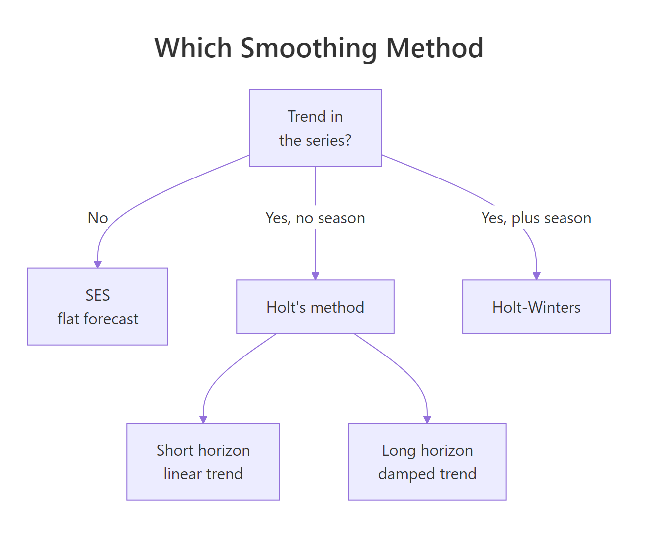
Figure 2: Choosing between SES, Holt, damped Holt, and Holt-Winters.
To see the seasonal failure for yourself, apply Holt to the monthly AirPassengers series, which has both a strong trend and a strong yearly cycle. Watch the last few forecasts.
The forecast climbs smoothly (446, 448, 450, 451) with no hint of the sharp summer peaks and winter troughs that define this series. Holt captured the upward trend but erased the season, which would badly mislead anyone planning around monthly demand.
On a genuine trend-only series, though, Holt earns its keep. Here we split airmiles into a training period and a test period, then compare Holt, damped Holt, SES, and a random-walk-with-drift baseline by their RMSE on the held-out years.
Both Holt variants beat SES by a wide margin on this trending data: SES posts a test RMSE of 7,364 against Holt's 1,575, because SES flattens a series that is clearly climbing. The damped version does best of all here (1,124), a reminder that damping is worth trying, not just for very long horizons.
ses() sets its alpha close to 1, the level is tracking each latest observation almost exactly, which usually means the series has a pattern SES cannot capture, often a trend. That is your cue to fit holt() and let a real trend term do the work.Try it: Apply holt() to the monthly co2 series (Mauna Loa atmospheric CO2, which also has a strong trend and a yearly cycle) twelve steps ahead, and check the last four forecasts for any seasonal ripple.
Click to reveal solution
Explanation: The four forecasts rise by a near-constant step with no up-and-down swing, so Holt has ignored the strong yearly cycle in co2 entirely. For a seasonal series like this you would reach for Holt-Winters, which adds a seasonal term on top of the level and trend.
Complete Example: forecasting Australian residents
Let's put every piece together on a fresh dataset. The built-in austres series records the number of Australian residents (in thousands), measured each quarter from 1971 to 1993. It has a strong, smooth upward trend and no meaningful seasonal cycle, which makes it a natural fit for Holt's method. We fit the model and read its parameters first.
The optimiser settles on alpha = 0.9999, meaning the level hugs the latest observation almost exactly, which makes sense for a population count that changes little from one quarter to the next. The trend dial beta = 0.4421 is moderate, giving a slope that responds to genuine shifts in the growth rate. Now check the fit.
The MAPE of 0.049 says the fitted values are within about 0.05% of the actual residents, an almost perfect in-sample fit for such a smooth series. Because the trend is so strong and steady, it is worth asking whether damping changes the long-range forecast much.
Twelve quarters out the two forecasts differ by only about 74 thousand residents (18,176 versus 18,103), because the estimated damping is light. For a short horizon like this, either is fine. Finally, read the forecast and plot it.
The forecast rises by about 43 thousand residents each quarter, continuing the historical trend, with narrow prediction bands that reflect how regular the series is. That is the full loop: fit the model, inspect the dials, check the accuracy, weigh whether to damp, then read the forecast.
Practice Exercises
These capstone problems combine the ideas above. Each uses fresh variable names so nothing you ran earlier gets overwritten. Try them before opening the solutions.
Exercise 1: Does damping change a steep forecast?
The built-in uspop series records the US population (in millions) at each census from 1790 to 1970. Fit both a plain and a damped Holt model with a 5-step horizon. Compare the final forecasts, then read the damping factor.
Click to reveal solution
Explanation: Five steps out, the plain model forecasts 324.7 million while the damped model forecasts 298.2 million. The lower phi here (0.9237, more damping than airmiles had) bends the steep population trend down noticeably, which is exactly the behaviour you want when a fast-growing series cannot realistically keep accelerating forever.
Exercise 2: Rebuild the forecast from the final states
Show that the Holt forecast really is the final level plus the final trend. Using the fit object from the tutorial (Holt on airmiles), read the last level and last trend from the fitted states, then reconstruct the first two point forecasts by hand.
Click to reveal solution
Explanation: The final level (30,657) plus one trend (2,107) reproduces the first forecast, 32,764.31, and plus two trends reproduces the second, 34,871.30, exactly matching fit$mean. The forecast equation is not an approximation: it is precisely the final level extended by the final slope.
Exercise 3: Which model generalises best on airmiles?
Split airmiles into a training set (up to 1955) and a test set (1956 onward). Fit Holt, damped Holt, and SES on the training set, then compare their RMSE on the held-out years. Which would you trust for a trending series?
Click to reveal solution
Explanation: SES posts a test RMSE of 7,364 because it flattens a rising series, while both Holt variants stay under 1,600. Damped Holt wins here at 1,124. On trending data, a model with a trend term generalises far better than one without.
Frequently Asked Questions
What is the difference between Holt's method and simple exponential smoothing?
Simple exponential smoothing tracks a single quantity, the level, so its forecast is a flat line. Holt's method adds a second tracked quantity, the trend, and carries it forward, so its forecast is a sloped line. Put simply, SES answers "what is the level now?" while Holt answers "what is the level now, and how fast is it changing?"
What does the beta parameter do?
Beta is the smoothing dial for the trend, just as alpha is the dial for the level. A large beta lets the estimated slope react quickly to recent changes in direction; a small beta keeps the slope steady and smooth, leaning on its own history. Like alpha, beta lives between 0 and 1, and holt() estimates it for you by minimising squared error.
Why would I damp the trend?
An undamped Holt forecast projects the same slope forever, which often overshoots at long horizons because real growth tends to level off. Setting damped = TRUE multiplies the trend by a factor phi (just under 1) at each step, so the forecast line gradually flattens. Damping is the safer default whenever you forecast many steps ahead.
Can Holt's method handle seasonality?
No. Holt models a level and a trend only, so it will track the overall direction of a seasonal series but erase the repeating up-and-down pattern. For data with a season, use Holt-Winters (which adds a seasonal term) or let ets() choose the components automatically.
How is holt() related to HoltWinters() and ets()?
All three fit exponential smoothing models. Base R's HoltWinters() can fit Holt's linear trend (call it with gamma = FALSE to drop the seasonal part) but minimises errors slightly differently and lacks the tidy forecast object. The forecast package's holt() is a friendly wrapper around ets() restricted to the trend model, known as ETS(A,A,N): additive error, additive trend, no season. Use holt() when you specifically want a trend forecast, and ets() when you want the software to compare model forms for you.
Summary
Holt's method is simple exponential smoothing plus a trend: two levels of smoothing, two dials, and a forecast that follows a straight line instead of a flat one. Everything flows from the level and trend equations.
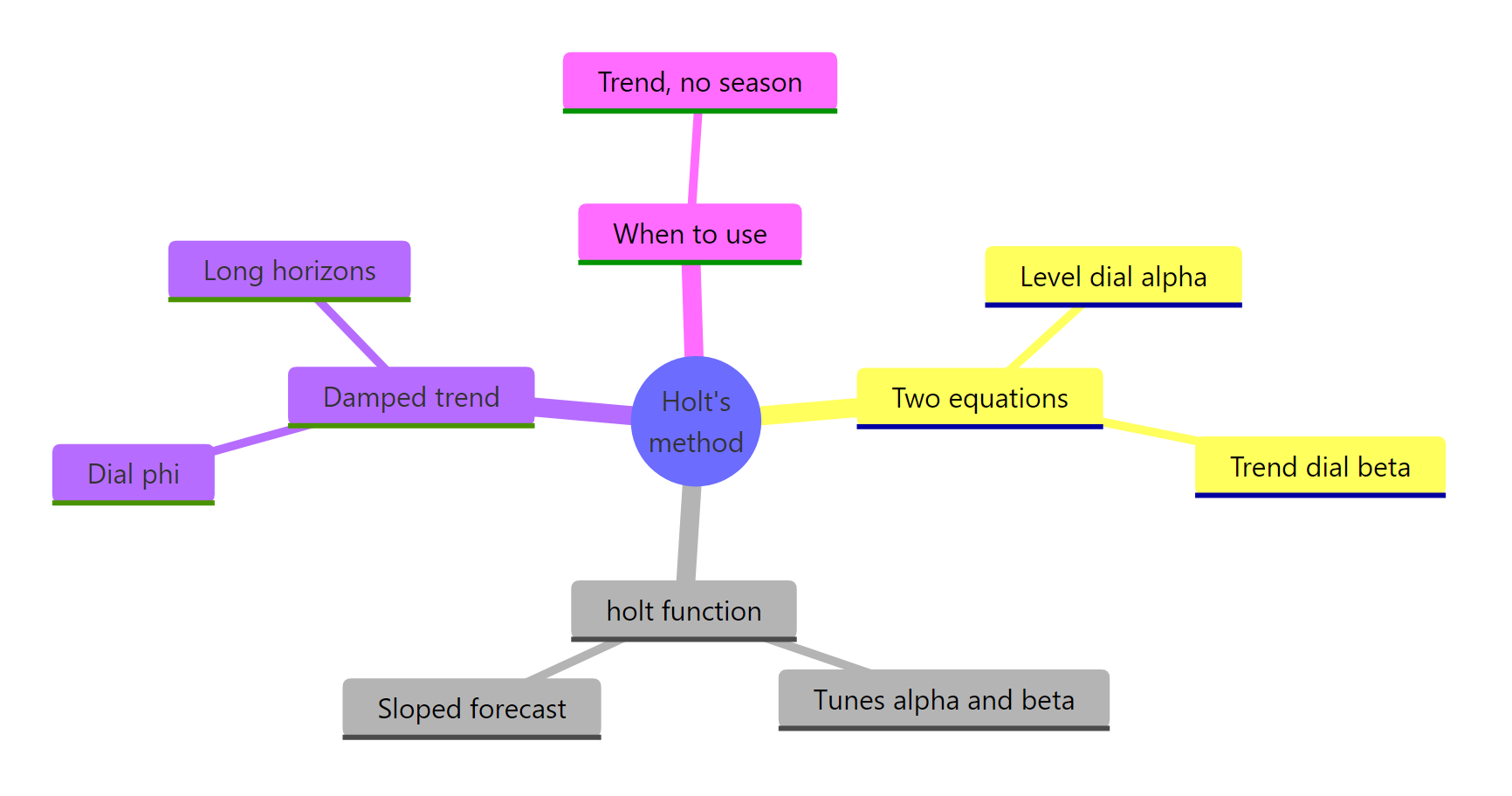
Figure 3: The moving parts of Holt's method in R.
| Idea | What to remember |
|---|---|
| The model | Level alpha * y + (1 - alpha) * (old level + old trend), trend smooths the observed slope, forecast is level + h * trend |
| Alpha | The level dial (0 to 1); high means the level follows recent data closely |
| Beta | The trend dial (0 to 1); high means the slope reacts fast, low means it stays smooth |
| holt() | Picks alpha, beta, and the starting states by minimising squared error |
| Damped trend | damped = TRUE multiplies the trend by phi each step so long-range forecasts flatten |
| When to use it | A series with a trend but no seasonality; use SES if flat, Holt-Winters if seasonal |
The holt() function packages all of this into one call: it fits the level and trend, tunes both dials, and returns a forecast whose sloped line continues the trend of your data. Reach for it whenever a series is clearly climbing or falling but not repeating a seasonal cycle.
References
- Hyndman, R.J. & Athanasopoulos, G. Forecasting: Principles and Practice, 2nd edition, Section 7.2: Trend methods (Holt's linear trend). Link
- Hyndman, R.J. & Athanasopoulos, G. Forecasting: Principles and Practice, 3rd edition, Section 8.2: Methods with trend. Link
- Hyndman, R.J. et al. forecast package documentation,
ses(),holt(), andhw()reference. Link - Holt, C.C. Forecasting seasonals and trends by exponentially weighted moving averages. International Journal of Forecasting, 20(1), 5-10 (2004; originally 1957). Link
- NIST/SEMATECH e-Handbook of Statistical Methods, Section 6.4.3.3: Double Exponential Smoothing. Link
- forecast package on CRAN. Link
- R Core Team.
airmilesandaustresdatasets, R datasets package documentation. Link
Continue Learning
- Exponential Smoothing in R: the parent lesson on simple exponential smoothing, the level-only base case that Holt's method extends.
- ETS Models in R: the
ets()function generalises Holt, choosing the error, trend, and seasonal components automatically. - Holt-Winters in R: add a seasonal term on top of the level and trend for series that repeat a yearly or weekly cycle.