Forecast Reconciliation in R: Bottom-Up to Middle-Out

Forecast reconciliation is the step that makes a set of forecasts add up. The oldest family of methods, bottom-up, top-down and middle-out, all do it the same way: pick one level of the hierarchy, trust it completely, and rebuild every other level from it. This tutorial shows exactly what each one computes, verifies the arithmetic by hand, and measures which one actually forecasts better.

Why does one hierarchy give you three different totals?

A forecasting model does not know that Tasmania and Western Australia are supposed to add up to a national total. It just sees numbers. Fit one model per series and you get one answer for the total, a different answer from summing the states, and a third from summing the regions. Let's build that hierarchy and watch the three answers disagree.

The tourism dataset ships inside the tsibble package. It records quarterly overnight trips in Australia from 1998 to 2017, broken down by region, state and trip purpose. We will keep two states, Tasmania and Western Australia, because they have five regions each. That gives a small hierarchy we can print in full and check by hand.

Three things happened in that block. First, summarise() added up the four trip purposes inside each region and quarter, because purpose is a breakdown we do not want here. Second, as_tsibble() declared the time column (index = Quarter) and the columns that identify a series (key = c(State, Region)). Third, and this is the important one, aggregate_key(State / Region, ...) read the slash as "Region nests inside State" and physically added every implied total as extra rows.

The <aggregated> label marks those added rows. A row with <aggregated> in both columns is the grand total across both states. options(pillar.sigfig = 5) just asks tibbles to print five significant digits instead of the default three, so we can read the decimals that the rest of this tutorial depends on.

Let's see exactly which series now exist.

Thirteen series in three tiers: one grand total, two states, ten regions. We started with ten. The other three were created by aggregate_key().

That is the structure. Now we fit a model to every one of those thirteen series independently and forecast one quarter ahead. ETS() fits an exponential smoothing model, and model() applies it to each series separately. Nothing in this step knows the hierarchy exists.

The label() helper collapses the two key columns into one readable name so the tables in this tutorial stay narrow: a region keeps its own name, a state row shows the state, and the grand total shows TOTAL. The .mean column that forecast() produces is the point forecast, which is the single number you would put in a plan. These are called base forecasts: the raw, unreconciled output of thirteen independent models.

Now the punchline. Ask this hierarchy for next quarter's total three different ways.

Each element picks a different set of rows and adds them up. top_model is the single forecast from the model fitted to the grand-total series. state_sum adds the two state forecasts. region_sum adds the ten region forecasts. We also stash the top-level number in top_fc, because every top-down calculation later in this tutorial starts from it.

Three answers to one question: 3942.6, 3854.6 and 3816.3. The spread is about 126 thousand trips, roughly 3 percent. Nothing in R warned us. Every model was fitted correctly; they simply were never told they had to agree.

Forecasts that do add up correctly are called coherent. Turning an incoherent set into a coherent one is reconciliation. The question this tutorial answers is which of the three numbers above you should build the coherent set around.

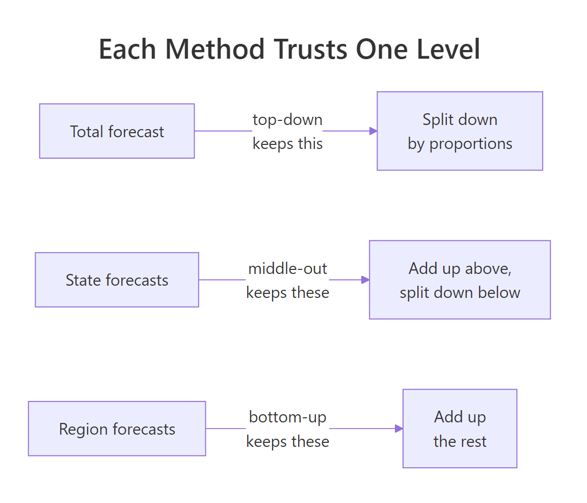
Figure 1: Each single-level method keeps one level and rebuilds the rest.

How does bottom-up reconciliation work?

Bottom-up is the method you would invent yourself in about ten seconds. Trust the smallest series, the ones closest to the actual thing being counted, and add them up. No proportions, no matrices, no assumptions.

Let's do it manually first, so there is no mystery about what the function does. We take the ten region forecasts, add them within each state, and then add the two state numbers.

The filter() keeps only rows whose Region is a real region, dropping the three aggregate rows. summarise(.by = State) then adds the five region forecasts inside each state. Tasmania comes to 1076.8 and Western Australia to 2739.5, and those two add to 3816.3.

Notice what we never used: the model fitted to Tasmania, the model fitted to Western Australia, and the model fitted to the grand total. Three of our thirteen models contributed nothing. Bottom-up throws them away.

Now the same thing with fable. The reconcile() step sits between model() and forecast() and attaches a reconciliation method to the existing models.

reconcile(bu = bottom_up(base)) says "take the column of models called base and add a second column called bu that reconciles them bottom-up". forecast() then produces both sets at once, which pivot_wider() turns into side-by-side columns.

Read the two columns against each other. Rows 1 to 5 and 7 to 11 are the regions, and they are identical in both columns. Rows 6, 12 and 13 are the aggregates, and they moved: Tasmania from 1120.2 to 1076.8, Western Australia from 2734.5 to 2739.5, the total from 3942.6 to 3816.3. Those are exactly the numbers we computed by hand.

Also note that the two adjustments went in opposite directions. Tasmania's own model was optimistic relative to its regions, Western Australia's was pessimistic. Bottom-up applies the same rule in both cases: replace the aggregate forecast with the sum of the series below it, whichever direction that moves the number.

The cost is noise. Small series are erratic, and adding ten erratic forecasts gives you an erratic total, even when the total itself was smooth and easy to model. We will measure that cost against a real holdout later in this tutorial.

How does top-down split a total into its parts?

Top-down is the mirror image. Trust the total, then break it into pieces. The only question is what share each bottom series should get.

Those shares are called disaggregation proportions, written $p_1, p_2, \dots, p_m$ for the $m$ bottom-level series. They have to sum to 1, otherwise the pieces would not add back up to the whole. Given the top-level forecast $\hat{y}_h$, every bottom series gets

$$\tilde{y}_{j,h} = p_j \, \hat{y}_h$$

Where:

• $\tilde{y}_{j,h}$ = the reconciled forecast for bottom series $j$, $h$ steps ahead
• $\hat{y}_h$ = the base forecast for the grand total, $h$ steps ahead
• $p_j$ = the share of the total that series $j$ gets, with $\sum_j p_j = 1$

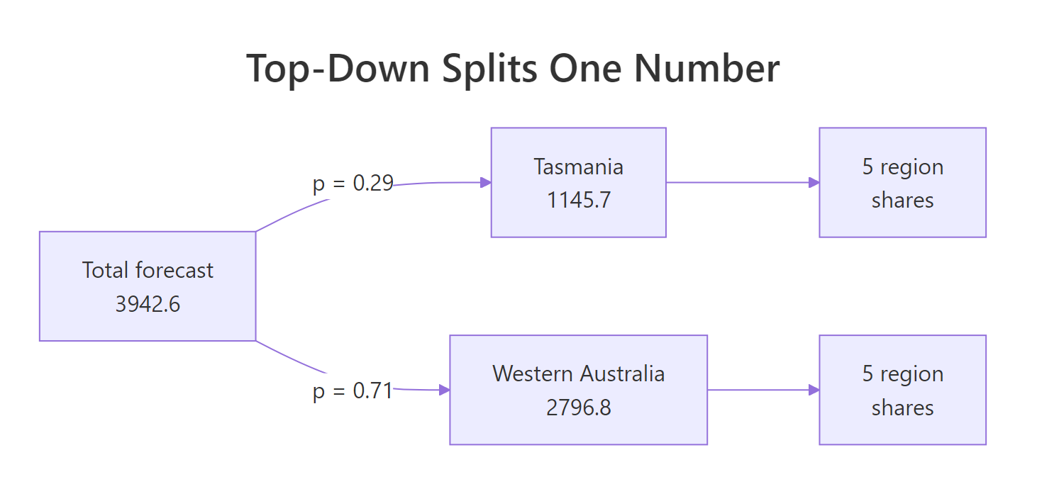
Figure 2: Top-down splits one number down the hierarchy using proportions.

So where do the $p_j$ come from? The two classical answers both look at history, and they differ in a way that sounds like hair-splitting but is not.

Average of historical proportions. For each quarter, work out what share this region took of that quarter's total, then average those shares across all quarters.

$$p_j = \frac{1}{T}\sum_{t=1}^{T}\frac{y_{j,t}}{y_t}$$

Proportions of historical averages. Average the region across all quarters, average the total across all quarters, then divide one by the other.

$$p_j = \frac{\sum_{t=1}^{T} y_{j,t} / T}{\sum_{t=1}^{T} y_t / T}$$

Where, in both formulas:

• $y_{j,t}$ = the observed value of bottom series $j$ in period $t$
• $y_t$ = the observed grand total in period $t$
• $T$ = the number of historical periods

The difference is the order of the division and the averaging. The first treats every quarter as one equal vote regardless of how big that quarter was. The second lets big quarters count for more, because it averages the raw values first. Let's compute both.

Follow the two paths. totals is the observed grand total in each of the 80 quarters. shares attaches that total to every region row and divides, giving each region's share in each quarter. Then p_ap averages those 80 shares per region, which is the first formula. p_pa instead averages each region's raw trips and divides by the average total, which is the second formula.

Experience Perth takes about 31 percent of the two-state total either way. The two columns are close but not equal, and we will quantify that gap in a moment.

Now let's confirm that the package is doing exactly this arithmetic. We run top_down() twice, once per method, and compare against our hand-computed numbers multiplied by the top-level forecast.

We multiplied each hand-computed proportion by top_fc, the 3942.6 grand-total forecast, then joined fable's own output alongside and took the largest absolute difference. Both gaps are exactly zero across all ten regions.

That is worth pausing on. The formulas above are not an approximation of what top_down() does; they are what it does. Here are the numbers themselves.

Column by column, hand and package agree to the last displayed digit. Now compare East Coast against its own base forecast of 153.6: top-down puts it at about 129 instead. East Coast's own fitted model contributed nothing to that figure. It came entirely from the grand total multiplied by a historical share.

Which top-down proportions should you use?

We now have two ways to compute $p_j$ and a third still to meet. Start by asking how much the first two actually differ, because if the answer is "barely", the choice does not deserve much of your attention.

We converted each proportion to a percentage, took the difference between the two methods, and sorted by the largest absolute move. The biggest disagreement anywhere in the hierarchy is 0.22 percentage points, on Experience Perth. On a total of 3942.6 that is about 9 thousand trips out of nearly 4 million.

So the choice between the two historical variants is close to a coin flip in practice. Both share a much more serious weakness: the proportions are frozen. They are computed once from the whole history and then applied to every future horizon. A region whose share has been climbing steadily for twenty years gets its twenty-year average share, not the share it is heading towards.

That is the problem the third method solves. Forecast proportions compute the shares from the base forecasts themselves rather than from history, level by level. For a bottom series $j$ in a hierarchy with $K$ levels:

$$p_j = \prod_{\ell=0}^{K-1} \frac{\hat{y}_{j,h}^{(\ell)}}{\hat{S}_{j,h}^{(\ell+1)}}$$

Where:

• $\hat{y}_{j,h}^{(\ell)}$ = the base forecast of the node that sits $\ell$ levels above series $j$
• $\hat{S}_{j,h}^{(\ell+1)}$ = the sum of the base forecasts of all the children of the node $\ell + 1$ levels above $j$
• $K$ = the number of levels in the hierarchy

That product notation hides a very simple recipe, so let's just perform it. Our hierarchy has two levels below the top. Step one: split the grand total between the two states in proportion to their own base forecasts. Step two: split each state's resulting number among its five regions in proportion to their base forecasts.

Read the two share columns. state_share is each state's base forecast divided by the sum of the two state base forecasts, so Tasmania gets 0.2906 and Western Australia 0.7094. region_share is each region's base forecast divided by the sum of the five regions in its own state, which is what .by = State inside mutate() arranges. Multiplying the grand total by both shares walks the number down two levels.

Every base forecast in the hierarchy influenced the answer. That is the crucial difference from the historical variants, which only ever looked at the top model and at raw history. Let's put all three variants next to each other.

Row 13 is the fixed point of the whole family: all three variants reproduce 3942.6, the base total, unchanged. Rows 1 to 12 tell the interesting story. The td_ap and td_pa columns track each other closely, as we already measured. The td_fp column sits somewhere else entirely, and consistently closer to base, because it was built from those base forecasts.

Look at Experience Perth in row 11. Its own model said 1084.4. The historical variants pushed it up past 1224, because Perth has historically taken a bigger share than its current forecast implies. Forecast proportions landed at 1107.1, much nearer its own model. That is the trend-tracking behaviour the historical variants cannot produce.

One more property of the whole top-down family is worth knowing, and it is easy to miss because everything above looks so reasonable. A forecast is unbiased when its errors average out to zero over many forecasts: it comes out too high about as often, and by about as much, as it comes out too low. Even when every base forecast is unbiased in that sense, top-down reconciled forecasts are not guaranteed to be. Splitting a total by fixed shares introduces a distortion whenever the shares themselves are uncertain, and no choice of $p_j$ removes it. Bottom-up has no such problem, because summing unbiased forecasts gives an unbiased sum.

What does middle-out do differently?

Deep hierarchies often have one level where the data is simply better than anywhere else. Individual stores are noisy, the national total is too coarse to plan against, but regions have enough volume to be stable and enough detail to be useful. Middle-out is built for that situation.

The recipe combines the two methods you have already seen. Pick a level. Above it, go bottom-up: add the chosen level's forecasts upward. Below it, go top-down: split each chosen-level forecast among its children using forecast proportions.

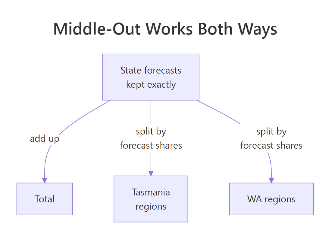
Figure 3: Middle-out adds up above the chosen level and splits down below it.

In fable the function is middle_out(), and it takes a split argument naming the level to anchor on. Level 1 is the first level below the grand total, which in our hierarchy is State.

Rows 6 and 12 did not move: Tasmania stayed at 1120.2 and Western Australia at 2734.5. That is the anchored level, preserved exactly, the same way bottom-up preserved the regions. Row 13 became 3854.6, which is simply 1120.2 plus 2734.5, the bottom-up step. Every region row moved, because each one was regenerated from its state's number.

Notice the direction of the region moves. Tasmania's regions all went up, because Tasmania's own model was higher than the sum of its regions. Western Australia's all went down slightly, for the opposite reason. Let's verify that this is really the recipe, rather than trusting the label on the function.

We reused region_share, each region's base forecast as a fraction of its state's five regions, and multiplied it by that state's own base forecast instead of by a share of the grand total. Ten rows, ten exact matches. Middle-out below the anchor is precisely top-down with forecast proportions, started one level lower.

Now a practical trap. The widely-read textbook description of this function uses a signature that current fabletools does not accept. If you copy middle_out(base, level = 1, method = "forecast_proportions") from a tutorial, here is what happens.

tryCatch() runs the expression and, if it raises an error, hands the error object to the handler function instead of stopping the session. We print the message with cat() so you can read it. The message says exactly what is wrong: middle_out() has no level argument. The real signature is middle_out(models, split = 1), with no method argument at all, because the downward step always uses forecast proportions.

What do all three methods have in common?

You have now seen three recipes that look quite different: adding upward, splitting by historical shares, splitting by forecast shares. They are all the same operation with one ingredient swapped.

Every reconciliation method in fable computes

$$\tilde{y}_h = S G \hat{y}_h$$

Where:

• $\hat{y}_h$ = the vector of all base forecasts, one per series in the hierarchy
• $G$ = a matrix that maps those base forecasts down to a set of bottom-level values
• $S$ = the summing matrix, which adds those bottom-level values back up to fill in every aggregate
• $\tilde{y}_h$ = the vector of reconciled, coherent forecasts

$S$ is fixed the moment you decide the shape of the hierarchy. It contains no choices. The method is entirely the $G$ matrix. Let's build both by hand and multiply them, which is the most direct way to see what "the method is $G$" actually means.

Our thirteen-series hierarchy would need a 10 by 13 matrix, too wide to read on screen. So we shrink to Tasmania alone: one total and five regions, six series. Same ideas, matrices that fit.

The short lookup swaps the long region names for abbreviations so the matrices print in a readable width. ord fixes the order of the six series, total first and then the five regions, and yhat is the base-forecast vector in that order. These are the same Tasmania numbers you saw earlier, now as a plain named vector ready for matrix algebra.

Here is the summing matrix. Six rows, one per series in the hierarchy, and five columns, one per bottom series.

Read row by row. The Total row is all ones, meaning the total is the sum of all five regions. Each region row is a single one in its own column, meaning a region is just itself. That is the entire hierarchy encoded as arithmetic, and it never changes no matter which method you pick.

Now the bottom-up $G$. Its job is to answer "given all six base forecasts, what are the five bottom-level values?" Bottom-up's answer is "ignore the total, keep the five regions as they are".

A zero column for the total, then an identity matrix for the regions. "Discard the top forecast, copy the bottom ones." Multiply it out and compare against what fable produced.

%*% is R's matrix multiplication operator, and R evaluates it left to right: $G$ turns the six base forecasts into five bottom values, then $S$ expands those five back into all six coherent forecasts. Two identical rows. Six lines of matrix algebra reproduced the package exactly.

Now swap in top-down's $G$ and change nothing else.

pv holds the proportions-of-historical-averages shares for Tasmania's five regions, computed the same way as before. They occupy the Total column, and every other column is zero. In words: "take the total, multiply it by these shares, ignore all five region forecasts."

Identical again. Same $S$, same $\hat{y}$, same multiplication. The only thing that changed between the two results was thirty numbers in a matrix.

Which method actually forecasts best?

Everything so far has been mechanics. Now we measure. Reconciliation costs nothing to try, since it never refits a model, so there is no excuse for guessing.

The test is a holdout. Train on data up to the end of 2015, forecast the eight quarters of 2016 and 2017, and score those forecasts against what actually happened. Crucially, we score each level separately, because a method that helps at the top can hurt at the bottom.

yearquarter("2015 Q4") converts that piece of text into a quarterly date of the same type as the Quarter column, which is what lets filter() compare the two. The header then tells the story: 52 keys, which is thirteen series times four methods, and 416 rows, which is 52 times the eight-quarter horizon. All four sets of forecasts came out of one forecast() call, because reconciliation is a cheap linear adjustment applied after the models are already fitted.

Now score them. accuracy() compares each forecast against the full dataset and returns the standard error measures per series, which we group into the three levels and average.

is_aggregated() is a tsibble helper that tests whether a key value is one of the totals aggregate_key() created, which is how we sort the thirteen series into Total, State and Region. RMSE is the root mean squared error in the same units as the data, thousands of trips, so lower is better.

Middle-out won at the total by a wide margin, 143.6 against the base 179.8, and it also won at the region level. Bottom-up improved the total a little and hurt the state level badly. Top-down was the worst option at both lower levels here.

But look more carefully at three of those numbers. Bottom-up scored 52.3 at Region and so did base. Top-down scored 179.8 at Total and so did base. Middle-out scored 156.3 at State and so did base. Those are not coincidences.

Zero to six decimal places, once in each column, and each zero sits on a different row. Bottom-up's accuracy at the region level is not merely similar to the base forecast's, it is the base forecast. Same for top-down at the total and middle-out at the state level.

This is the whole argument of the tutorial visible as three zeros. Each method has one level it copies verbatim and cannot possibly improve, and every gain or loss it delivers happens somewhere else.

When should you use each method?

The bake-off above was one hierarchy over one holdout window. Do not generalise from it. What does generalise is the structure, so here is the decision framed around what each method keeps and what it destroys.

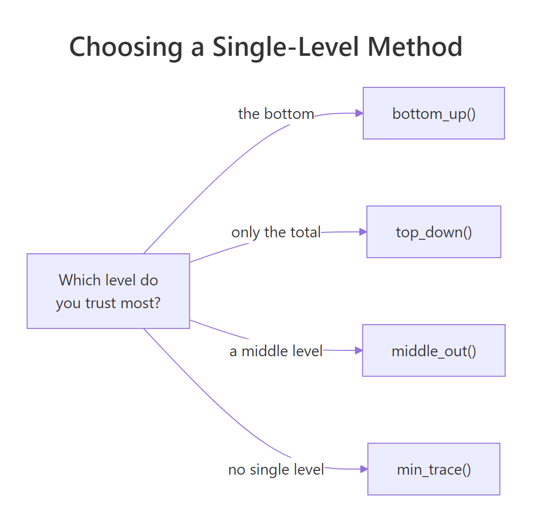
Figure 4: Which single-level method to reach for first.

The recurring question is which level is genuinely most forecastable. That is measurable before you reconcile anything. One quick proxy is the coefficient of variation, the standard deviation of a series divided by its mean, which says how much a series bounces around relative to its own size.

We computed the coefficient of variation for each of the thirteen series, then averaged within each level. It climbs steadily on the way down: 0.196 at the total, 0.248 at the states, 0.323 at the regions. Aggregation cancels out idiosyncratic noise, which is why totals are almost always the easiest series in a hierarchy to forecast.

That is the honest case for top-down, and the reason bottom-up can disappoint. It is also why the answer changes with the data: run this on a hierarchy where the bottom series are large and stable and the gap narrows or reverses.

There are situations where a single-level method is not a compromise but the correct choice:

• The bottom is brand new. Products launched last month have no history to model. Top-down gives them a share of a total you can actually forecast.
• The bottom is intermittent. Series that are zero most weeks break most forecasting models. Aggregate first, split afterwards.
• A number is mandated. If finance has committed to a total, top-down is the only family member that reproduces it untouched.
• You have no residuals. Judgemental forecasts, or numbers arriving from another team, come without an error history. Every single-level method works anyway; the modern alternatives do not.

When none of those constraints apply and you do have residuals, the case for a single-level method weakens sharply. Throwing away most of your models to satisfy a structural constraint is a strange trade when a method exists that uses all of them. That method is MinT, and it is the subject of the next tutorial in this series.

Complete Example: reconcile a fresh hierarchy three ways

Here is the whole workflow end to end on data we have not touched, Queensland and South Australia, in one uninterrupted pipeline. Raw quarterly data goes in, three coherent sets of forecasts come out.

Six verbs, in the order you will always use them: summarise() to collapse breakdowns you do not want, as_tsibble() to declare index and key, aggregate_key() to create the totals, model() to fit every series, reconcile() to attach the methods, forecast() to produce them all.

The output is the four quarters of 2018 at the grand-total level. The td column matches base in every row, because top-down never touches the total, on any horizon. Bottom-up sits consistently below both, and middle-out lands between them. The same structural pattern you saw on Tasmania and Western Australia reappears immediately on a completely different pair of states.

Practice Exercises

These combine several ideas from the tutorial. Every exercise is solvable with what you have already seen. Variables are prefixed my_ so they do not disturb anything defined above, and Exercise 3 reuses the hierarchy you build in Exercise 1.

Exercise 1: Reconcile a new pair of states two ways

Build a hierarchy from Victoria and South Australia with State / Region nesting, fit ETS() to every series, reconcile it with both bottom_up() and top_down(method = "forecast_proportions"), and report the one-step-ahead grand-total forecast for each of the three model columns.

Exercise 2: Rebuild top_down() from scratch with matrices

Reproduce top_down(method = "average_proportions") on the original thirteen-series hierarchy using only matrix algebra, then prove your result matches fable. You will need a 13 by 10 summing matrix and a 10 by 13 $G$ matrix whose only non-zero column holds the proportions from p_both$p_ap.

Order the series as TOTAL, then the two states, then the ten regions in the order they appear in base_mean.

Exercise 3: Run a bake-off and decide what to ship

Using my_hier from Exercise 1, train on data through 2015 Q4, forecast eight quarters with base, bottom_up(), top_down(method = "forecast_proportions") and middle_out(split = 1), and report mean RMSE by level. Then decide which method you would ship for Victoria and South Australia, and say why.

Frequently Asked Questions

Does making forecasts coherent also make them more accurate?

Not on its own. Coherence is a constraint on the numbers, not new information about the future, so reconciliation mostly moves accuracy around the hierarchy rather than adding it. In the bake-off above, bottom-up improved RMSE at the total from 179.8 to 172.8 and made the state level clearly worse, from 156.3 to 189.3. Score the methods on a holdout at the level you actually plan on, rather than assuming that adding up correctly means forecasting well.

If I only remember one of these methods, which should it be?

Bottom-up. It needs nothing but the bottom-level point forecasts, it works on every hierarchy shape, it never makes the bottom level worse, and it has no arguments to get wrong. It is the sensible default when you have real volume in the bottom series.

Can I use top_down() on a grouped structure?

No. If you build a crossed structure with aggregate_key(State * Purpose, ...), where two attributes cut across each other instead of nesting, top_down() stops with the message "Top down reconciliation requires strictly hierarchical structures". The reason is that a grouped structure has more than one path from the bottom to the total, so there is no single set of proportions to split by. middle_out() has the same restriction. bottom_up() works fine, because summing upward is well defined no matter how many paths there are.

Do these methods reconcile prediction intervals, or only the point forecasts?

The whole distribution. The Trips column in a fable is a distribution, not a number, and reconcile() acts on it. On the hierarchy in this tutorial the base 80 percent interval for the total was [3530.7, 4354.4] and the bottom-up one was [3565.1, 4067.4], so the reconciled interval is both shifted and considerably narrower.

Does reconciliation refit any models?

No. Every method here is a linear transformation applied to forecasts that already exist, which is why reconcile() sits after model() and costs essentially nothing. Adding a fourth or fifth method to the same call adds no model fitting at all, so there is no reason to guess which one is best when you can score them all.

Does any of this depend on using ETS?

No. Swap ETS(Trips) for ARIMA(Trips) and everything works identically, because reconciliation only ever sees the forecasts. On this hierarchy an ARIMA base gives a total of 3773.6 and its bottom-up reconciliation gives 3716.4, the same structural relationship as with ETS but different numbers.

Why is my middle_out() call asking me to file a bug report?

You almost certainly passed a split that points at the bottom level of the hierarchy. There is nothing below the bottom to split into, and rather than saying so, fabletools raises an internal error inviting a bug report. Anchor on a genuine middle level, and use bottom_up() if the bottom is what you meant.

Can reconciliation turn a positive forecast negative?

Bottom-up cannot, because it only adds non-negative numbers together. Top-down and middle-out cannot either, as long as the proportions are positive, because they multiply a positive total by fractions. Negative reconciled forecasts do appear with methods that subtract, such as MinT, and they are a known nuisance on low-count series.

Summary

The three classical methods, in one table:

The ideas worth carrying away:

• Incoherence is silent. Thirteen correctly fitted models gave three different answers for the same total, 3942.6, 3854.6 and 3816.3, and nothing warned us.
• Every method is $\tilde{y} = SG\hat{y}$. $S$ is fixed by the hierarchy shape; $G$ is the entire method. Bottom-up, top-down and middle-out differ only in which columns of $G$ are non-zero.
• The preservation identity is structural. Each method's accuracy at the level it trusts is identical to the base forecast's, to the last decimal, on every metric.
• Top-down has three proportion variants. The two historical ones differed by at most 0.22 percentage points here, and both freeze the shares. forecast_proportions is the default because it tracks trends in the mix.
• Check the signature, not the textbook. It is middle_out(models, split = 1). There is no level argument and no method argument.
• Always score by level. A single averaged accuracy number hides the whole trade, which is always "better here, worse there".

References

1. Hyndman, R.J. and Athanasopoulos, G. - Forecasting: Principles and Practice, 3rd edition. Chapter 11.2: Single level approaches. Link
2. Hyndman, R.J. and Athanasopoulos, G. - Forecasting: Principles and Practice, 3rd edition. Chapter 11.1: Hierarchical and grouped time series. Link
3. fabletools reference - top_down(): top-down forecast reconciliation. Link
4. fabletools reference - bottom_up(): bottom-up forecast reconciliation. Link
5. fabletools reference - middle_out(): middle-out forecast reconciliation. Link
6. Athanasopoulos, G., Ahmed, R.A. and Hyndman, R.J. - Hierarchical forecasts for Australian domestic tourism. International Journal of Forecasting 25(1), 146-166 (2009). Link
7. Hyndman, R.J., Ahmed, R.A., Athanasopoulos, G. and Shang, H.L. - Optimal combination forecasts for hierarchical time series. Computational Statistics and Data Analysis 55(9), 2579-2589 (2011). Link
8. Athanasopoulos, G., Hyndman, R.J., Kourentzes, N. and Panagiotelis, A. - Forecast reconciliation: a review. International Journal of Forecasting 40(2), 430-456 (2024). Link

Continue Learning

• Hierarchical and Grouped Time Series in R: Reconciliation - how to build hierarchies with aggregate_key(), what the summing matrix encodes in full, and how grouped structures differ from nested ones.
• fable in R: Tidy Time Series Forecasting with tsibble - the tsibble and fable foundations underneath every code block here, including how model(), mables and fables fit together.
• Forecast Accuracy in R: MAE, RMSE, MAPE, and MASE - what the RMSE and MASE numbers in the bake-off actually measure, and which one to believe when they disagree.