SARIMA in R: How to Fit Seasonal ARIMA Models
SARIMA (Seasonal ARIMA) is an ARIMA model with an extra set of terms that repeat every season, written ARIMA(p, d, q)(P, D, Q)[m]. The lowercase part handles short-term structure; the uppercase part handles the pattern that returns every m steps (m = 12 for monthly data). In R you fit one with Arima() or auto.arima() from the forecast package.
What is a SARIMA model, and how does it extend ARIMA?
Sales jump every December. Temperatures climb every summer. Electricity demand peaks every weekday evening. A huge share of real time series repeat on a fixed calendar, and a plain ARIMA model cannot see that repeat. SARIMA fixes this by adding a second set of ARIMA terms that work at the seasonal lag instead of the neighbouring one. The fastest way to see it is to point R at a famously seasonal series and let it pick a model on its own.
We will use the built-in AirPassengers series: monthly totals of international airline passengers from 1949 to 1960. Let's load the forecast package and ask auto.arima() to choose a model.
Look at the model label: ARIMA(2,1,1)(0,1,0)[12]. That second bracket of numbers is new. A plain ARIMA gives you three numbers; a SARIMA gives you seven. R detected that this series is monthly, added a seasonal piece, and even chose to difference it once at the seasonal lag (the 1 in the middle of (0,1,0)). By the end of this tutorial you will be able to read every number in that label and fit a model like it yourself.
If ARIMA on its own is still fuzzy, here is the one-line recap: an ARIMA(p, d, q) model predicts each value from its own recent values (the AR part, order p), works with changes instead of raw levels to remove trend (the I part, order d), and learns from its own recent forecast errors (the MA part, order q). Our ARIMA in R tutorial walks through those three ideas from scratch if you want a refresher.
SARIMA keeps all of that and adds three matching seasonal numbers plus the season length. Here is what all seven mean.
| Part | Symbol | Name | What it captures |
|---|---|---|---|
| Non-seasonal | p, d, q | AR, I, MA | Month-to-month structure, same as ARIMA |
| Seasonal | P, D, Q | Seasonal AR, I, MA | The pattern that returns every season |
| Period | m | Season length | Steps in one full cycle (12 for monthly) |
The diagram below shows how the label splits into those three groups.
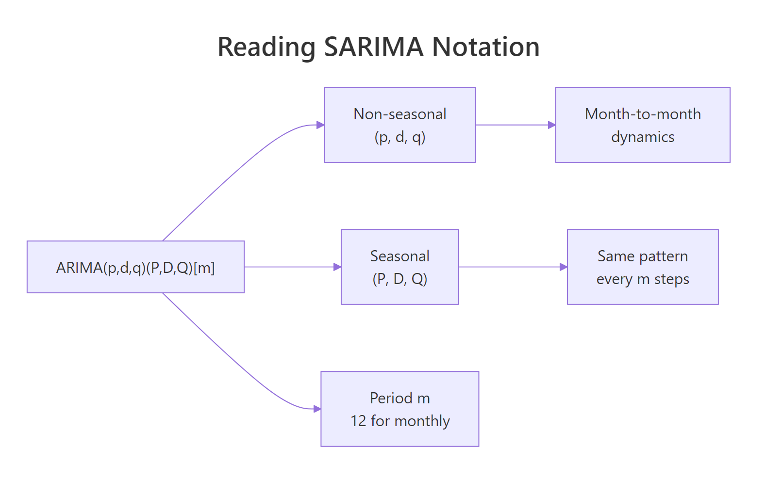
Figure 1: The SARIMA label splits into a non-seasonal part, a seasonal part, and the period m.
How did R know the season was 12 steps long? Because AirPassengers is stored as a monthly time series, and R reads its frequency directly.
The first line confirms the season is 12 observations long. The second shows the first twelve months of 1949, and you can already spot the shape: a rise into the summer, a dip in the autumn. That yearly rhythm repeats for every one of the twelve years in the data, and capturing it is exactly what the seasonal terms are for.
Try it: Fit an automatic model to the built-in USAccDeaths series (monthly accidental deaths in the US) and read off its (P, D, Q)[m] seasonal orders.
Click to reveal solution
Explanation: R picks ARIMA(0,1,1)(0,1,1)[12]. The seasonal orders are P = 0, D = 1, Q = 1, and the period is 12. That (0,1,1)[12] seasonal part is so common it has a nickname you will meet later: the airline model.
Why does plain ARIMA fail on seasonal data?
Before adding seasonal terms, it helps to see what goes wrong without them. First, let's make the seasonal pattern concrete by averaging every January together, every February together, and so on. If the series is truly seasonal, those monthly averages will differ a lot.
The numbers tell the story. July and August average 351 passengers, while November averages 233. That is a swing of about 50% driven purely by the month of the year. Any model that ignores the calendar is throwing away one of the strongest signals in the data.
Now let's fit an ARIMA model that is forbidden from using seasonal terms, by passing seasonal = FALSE, and see how it copes.
R uses four AR terms and two MA terms to approximate the yearly cycle with short-term memory. Notice sigma^2 = 706.3 here versus 132.3 for the seasonal model in the first section. The error variance is more than five times larger. The non-seasonal model uses far more terms and still fits far worse.
The clearest proof of failure is in the residuals, which are the leftover errors after the model has done its best. A good model leaves residuals that look like random noise. If the residuals still carry a yearly pattern, the model missed the season. The Ljung-Box test checks exactly this: a small p-value means significant leftover structure.
The p-value is 1.643e-14, which is essentially zero. That tiny number is strong evidence that the residuals still contain a clear pattern at the yearly lag. The non-seasonal model removed the trend but left the entire seasonal signal behind, which means its forecasts will miss every summer peak and every winter trough.
Try it: Average the USAccDeaths series by calendar month to reveal its seasonal shape. Which months are highest?
Click to reveal solution
Explanation: July (month 7) is the deadliest with about 10,453 deaths, and February (month 2) is the lowest at about 7,284. The summer peak is a clear seasonal signal that a good model must capture.
What do the seasonal terms (P, D, Q)[m] mean?
The seasonal terms are the non-seasonal ones with a longer reach. Where p, d, and q look back one step, P, D, and Q look back one whole season. Let's take them one at a time, starting with the period that ties them together.
m is the season length, the number of steps in one full cycle. It is monthly data's 12, quarterly data's 4, and daily-with-weekly-pattern data's 7. You do not estimate m; you know it from the calendar and R usually reads it from the series frequency.
D is the number of seasonal differences. A seasonal difference replaces each value with the change from one season ago: this July minus last July, this August minus last August. That single operation cancels a stable yearly pattern, because the summer bump appears in both the current value and the value twelve months back, so subtracting removes it. Let's watch it work. The nsdiffs() function tells you how many seasonal differences a series needs, and ndiffs() does the same for ordinary differences.
R recommends one ordinary difference (d = 1) to remove the upward trend and one seasonal difference (D = 1) to remove the yearly cycle. Let's confirm the seasonal difference actually does its job by applying it and re-checking.
After one seasonal difference (lag = 12 means subtract the value twelve months ago), nsdiffs() returns 0. The seasonality is gone, which is exactly what D = 1 buys you inside a SARIMA model.
P is the seasonal AR order and Q is the seasonal MA order. They are the AR and MA ideas aimed at the seasonal lag. A seasonal AR term of order 1 says this July leans on last July's value. A seasonal MA term of order 1 says this July leans on last July's forecast error. Just like their lowercase cousins, you rarely need more than one or two of each.
m is set automatically. For data you import yourself, set it when you build the series, for example ts(x, frequency = 12) for monthly data.Try it: Find the seasonal period of the UKgas series (quarterly UK gas consumption). What value of m would a SARIMA model use for it?
Click to reveal solution
Explanation: UKgas is quarterly, so it has 4 observations per cycle and a SARIMA model would use m = 4. The seasonal terms would then reach back 4 quarters (one year) instead of 12 months.
How do you find the right seasonal orders from ACF and PACF?
You have two families of numbers to pin down: the differencing orders (d and D) and the term orders (p, q, P, Q). Differencing comes first, because you can only read the term orders off a stationary series, one whose statistical behaviour no longer drifts over time.
One quick preparation step matters for AirPassengers: the seasonal swings grow larger as the level rises. Taking a logarithm first stabilises that spread, turning a widening fan into an even band, which makes the model fit better. Let's find the differencing counts on the logged series.
So we need one ordinary difference and one seasonal difference, the same d = 1, D = 1 as before. Now apply both and inspect the autocorrelation plots. The autocorrelation function (ACF) measures how each value correlates with values at earlier lags; the partial autocorrelation function (PACF) does the same after removing the effect of the lags in between. ggtsdisplay() shows the differenced series alongside both plots at once.
Running that draws three panels. The differenced series at the top now hovers around a flat zero line with no drift and no obvious yearly wave, which confirms it is stationary. The ACF and PACF below it are where you read the seasonal orders, and there is a simple rule for that.
Look only at the seasonal lags, the multiples of 12 (lag 12, 24, 36). Ignore everything in between when deciding the seasonal orders. Then apply the same logic you use for non-seasonal terms, just at those seasonal positions.
- A single spike in the ACF at lag 12 that then dies away, paired with a slow decay in the PACF at seasonal lags, points to a seasonal MA term (
Q = 1). - A single spike in the PACF at lag 12, paired with a slow decay in the ACF at seasonal lags, points to a seasonal AR term (
P = 1).
For the logged AirPassengers, the ACF shows one clean negative spike at lag 12 and the PACF tapers off across the seasonal lags, which is the signature of a seasonal MA term. That is Q = 1. The diagram below captures the rule so you can reuse it on any series.
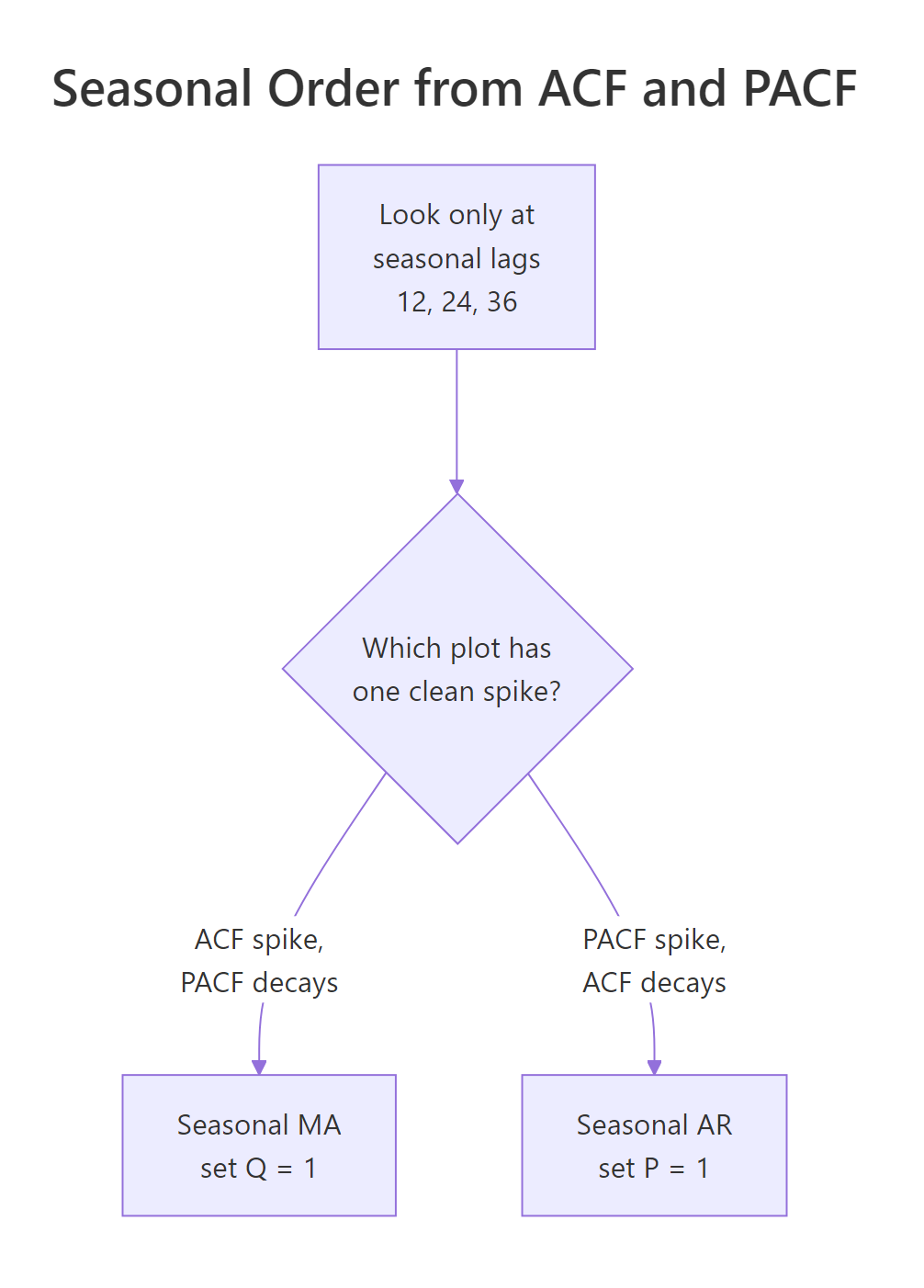
Figure 2: Reading seasonal AR versus seasonal MA from the ACF and PACF at seasonal lags.
ndiffs() and nsdiffs() functions use formal unit-root tests to pick d and D, which is more reliable than eyeballing. Use the ACF and PACF to sanity-check the result and to read the term orders, not to guess the differencing.Try it: Take one seasonal difference of USAccDeaths and confirm nsdiffs() drops to 0, proving one seasonal difference is enough.
Click to reveal solution
Explanation: With lag = 12 the seasonal difference cancels the yearly cycle, so nsdiffs() returns 0. One seasonal difference is enough, which means D = 1 for this series.
How do you fit a SARIMA model in R with auto.arima() and Arima()?
You now have all the orders for AirPassengers: d = 1, D = 1, Q = 1, and the classic choice for this data adds one non-seasonal MA term (q = 1) too. That gives ARIMA(0,1,1)(0,1,1)[12], the model so famous for this series that it is known as the airline model. Let's fit it by hand with Arima().
The Arima() function takes the non-seasonal orders in order = c(p, d, q) and the seasonal orders in seasonal = list(order = c(P, D, Q), period = m). The lambda = 0 argument tells R to fit on the log scale for us and back-transform automatically, so we do not have to log the data by hand.
The model has two coefficients. ma1 = -0.4018 is the ordinary moving-average term, correcting each month using last month's error. sma1 = -0.5569 is the seasonal moving-average term, correcting each month using the error from twelve months ago. Those two numbers, plus the two differences, are the whole model.
Now here is the satisfying part. Watch what auto.arima() picks when we give it the same log transform and let it search freely.
It lands on exactly the same model, the airline model, coefficient for coefficient. Your hand-reasoning from the ACF and PACF and R's automatic search agree. We can confirm they score identically by comparing their AICc, an information criterion where lower means a better trade-off between fit and complexity.
Identical scores, because they are the same model. This is the ideal outcome: you understand why the model has the terms it does, and you have an automatic tool that reproduces your reasoning and scales to series you have not studied by hand.
Here is how the airline model looks as an equation, now that you have seen its coefficients. Each factor below is one of the four things we chose. If formulas are not your thing, skip to the next section; the code above is all you need to fit the model.
$$(1 - B)(1 - B^{12})\, y_t = (1 + \theta_1 B)(1 + \Theta_1 B^{12})\, \varepsilon_t$$
Where:
- $B$ = the backshift operator, which steps back one period, so $B\,y_t = y_{t-1}$ and $B^{12} y_t = y_{t-12}$
- $(1 - B)$ = one ordinary difference, the
d = 1part - $(1 - B^{12})$ = one seasonal difference, the
D = 1part - $\theta_1$ = the non-seasonal MA coefficient, the
ma1above - $\Theta_1$ = the seasonal MA coefficient, the
sma1above - $\varepsilon_t$ = the unpredictable error at time $t$
lambda = 0, so their scores are comparable. Never compare an AICc from a logged fit against one from an unlogged fit; the numbers live on different scales.Try it: Fit the airline model ARIMA(0,1,1)(0,1,1)[12] to USAccDeaths by hand with Arima() and confirm it matches the model auto.arima() chose in the first section.
Click to reveal solution
Explanation: The seasonal = c(0, 1, 1) shorthand fills in (P, D, Q) and R reads the period from the series. The coefficients match auto.arima(USAccDeaths) from the first exercise exactly, because it is the same model.
How do you check the model and forecast the future?
Fitting a model is only half the job. Before you forecast, you have to confirm the model is adequate, and the check is the same one we used to condemn the plain ARIMA earlier: the residuals should look like random noise with nothing left over. The checkresiduals() function runs a Ljung-Box test and draws the residual diagnostics in one call.
The p-value is 0.233, comfortably above 0.05. Unlike the tiny p-value from the plain model, this one says we cannot reject the idea that the residuals are pure noise. The plot that accompanies this output shows residuals bouncing around zero, an ACF with no spikes poking past the blue bounds, and a roughly bell-shaped histogram. The model has captured the structure and left only randomness behind, so it is safe to forecast with.
Now for the payoff. The forecast() function projects the model forward; here we ask for 24 months, two full years ahead, and plot the result with autoplot().
The plot shows the historical series in one colour, the forecast continuing its upward trend, and a shaded fan around the forecast that widens as we look further out. That widening fan reflects growing uncertainty: the further ahead you predict, the wider the interval around the forecast. Notice the forecast keeps the seasonal shape, peaking each summer and dipping each winter, which is the whole reason we used a SARIMA model. Let's print the point forecasts to see the actual numbers.
Read across 1961: the model predicts the familiar summer peak (670 in July) and winter lull (426 in February), and read down and you see 1962 sitting higher than 1961, because the model also carried the long-run growth trend forward. Seasonality and trend, both projected in one model.
checkresiduals() returns a small p-value or shows a spike at the seasonal lag, the model is still missing structure, and the usual fix is to add a seasonal AR or seasonal MA term and refit. A clean residual check is your green light to forecast.Try it: Forecast the next 12 months of USAccDeaths using the airline model and print the point forecasts.
Click to reveal solution
Explanation: The forecast for 1979 mirrors the historical shape, peaking in July (10,907) and dipping in February (7,532). The SARIMA model projected the seasonal pattern one year forward.
Complete Example: Forecast airline passengers and measure the error
Let's put every step together on a real forecasting task and, crucially, measure how good the forecast actually is. The honest way to do that is to hide the last stretch of data, train the model on the rest, forecast the hidden part, and compare. We will train on everything through the end of 1958 and hold out 1959 and 1960 as a test set.
The window() function slices a time series by date. With the split in place, we fit the airline model on the training data only, forecast 24 months to cover the test period, and score the result with accuracy(), which reports error metrics on both the training and test sets.
Focus on the MAPE column, the mean absolute percentage error. On the held-out years the model is off by about 8.5% on average, forecasting two full years into the future it had never seen. The Test set error is larger than the Training set error of 2.6%, which is completely normal: a model always looks better on data it learned from than on data it must predict. An 8.5% error two years out on a genuinely seasonal series is a strong result.
For peace of mind, let's confirm the automatic search would have reached the same model on the training data.
Same ARIMA(0,1,1)(0,1,1)[12] structure, with coefficients estimated from the shorter training window. That is the full SARIMA workflow start to finish: spot the season, difference it away, read or search for the orders, fit, check residuals, forecast, and measure the error.
Frequently Asked Questions
What is the difference between (p, d, q) and (P, D, Q)? They are the same three ideas at two different reaches. The lowercase (p, d, q) act on neighbouring steps: p looks back one step, d differences one step, q uses the last step's error. The uppercase (P, D, Q) do the identical jobs but reach back one whole season of m steps: for monthly data that is 12 months, so P looks back to the same month last year.
Do I need both a regular difference and a seasonal difference? Often yes, and they remove different things. A regular difference (d = 1) removes a trend that carries over month to month; a seasonal difference (D = 1) removes a pattern that repeats every year. AirPassengers has both a rising trend and a yearly cycle, so it needs d = 1 and D = 1. Use ndiffs() for d and nsdiffs() for D, and rarely will either go above 1.
How do I set the season length m for my own data? R only reads m automatically when the series already carries a frequency, as the built-in datasets do. For data you import, set it when you build the series with ts(), for example ts(x, frequency = 12) for monthly data or ts(x, frequency = 4) for quarterly. If you leave the frequency at 1, R treats the data as non-seasonal and auto.arima() will never add seasonal terms.
When should I log the data before fitting a SARIMA model? Log the series when the seasonal swings grow wider as the level rises, as they do for AirPassengers. The lambda = 0 argument does this for you: it fits on the log scale and back-transforms the forecast automatically, so you never work with logged numbers by hand. If the swings stay a roughly constant size over time, you do not need it.
auto.arima() did not add any seasonal terms. What went wrong? The most common cause is that the series does not carry a frequency above 1, so R has no season length to work with. Check frequency(your_series); if it returns 1, rebuild the series with the correct frequency and refit. It is also worth setting stepwise = FALSE and approximation = FALSE, which make auto.arima() search more thoroughly at the cost of speed.
Practice Exercises
These capstone exercises combine several steps from the tutorial. Each uses its own variable names so it will not collide with the code above. Try each one before opening the solution.
Exercise 1: Fit automatically and prove the residuals are clean
Fit an automatic seasonal model to USAccDeaths, then run a Ljung-Box test on its residuals at lag 24. Decide whether the residuals look like white noise.
Click to reveal solution
Explanation: The p-value of 0.3484 is well above 0.05, so we cannot reject white noise. The airline model captured the structure in USAccDeaths, leaving only random residuals, so it is safe to forecast with.
Exercise 2: Backtest the model on held-out data
Split USAccDeaths so the training set runs through December 1977 and the test set is all of 1978. Fit the airline model on the training set, forecast 12 months, and report the test-set RMSE and MAPE with accuracy().
Click to reveal solution
Explanation: The test-set RMSE is about 289 deaths and the MAPE is 2.72%, so the model predicts the unseen year to within about 3% on average. The low test error confirms the airline model generalises well to this series.
Exercise 3: Prove that the seasonal terms actually help
Fit two automatic models to USAccDeaths, one with seasonal = FALSE and one with seasonal = TRUE, then compare their AICc values. Does the seasonal model win?
Click to reveal solution
Explanation: The seasonal model scores 857.32 against the non-seasonal model's 1141.70. Lower AICc is better, so the seasonal model wins by a wide margin, which is the numerical proof that the (P, D, Q) terms earn their place.
Summary
SARIMA extends ARIMA with a matching set of terms that operate one full season back instead of one step back. You spot the season, difference it away, read or search for the orders, fit with Arima() or auto.arima(), check the residuals, and forecast. The diagram below recaps that flow.

Figure 3: The six-step SARIMA workflow from plot to forecast.
Here is every SARIMA term in one place, with the R argument that controls it.
| Term | Meaning | Set in R with |
|---|---|---|
| p, d, q | Non-seasonal AR, differencing, MA | order = c(p, d, q) |
| P, D, Q | Seasonal AR, differencing, MA | seasonal = c(P, D, Q) |
| m | Season length (12 monthly, 4 quarterly) | Read from the series frequency |
| lambda = 0 | Fit on the log scale to stabilise variance | lambda = 0 |
The key takeaways to carry forward:
- Seasonal data needs seasonal terms. A plain ARIMA leaves the yearly pattern stranded in the residuals, and a Ljung-Box test at the seasonal lag will expose it.
- D removes the season, P and Q model what remains. One seasonal difference usually flattens a stable yearly cycle; then one seasonal AR or MA term captures the leftover seasonal correlation.
- Read only the seasonal lags when picking P and Q. An ACF spike at lag m points to seasonal MA; a PACF spike at lag m points to seasonal AR.
- auto.arima() is a reliable default, and when you understand the orders yourself, its output stops being a black box and becomes a confirmation.
References
- Hyndman, R.J. & Athanasopoulos, G. - Forecasting: Principles and Practice (2nd ed), Section 8.9: Seasonal ARIMA models. Link
- Hyndman, R.J. & Athanasopoulos, G. - Forecasting: Principles and Practice (3rd ed), Section 9.9: Seasonal ARIMA models. Link
- Hyndman, R.J. - forecast package:
Arima()reference. Link - Hyndman, R.J. - forecast package:
auto.arima()reference. Link - Box, G.E.P., Jenkins, G.M., Reinsel, G.C. & Ljung, G.M. - Time Series Analysis: Forecasting and Control, 5th Edition. Wiley (2015). The origin of the airline model.
- R Core Team -
stats::arimadocumentation. Link - Nau, R. - Seasonal ARIMA models (Duke University). Link
Continue Learning
- ARIMA in R: What AR, I, and MA Mean and How to Fit One - the non-seasonal foundation that SARIMA builds on, explained from scratch.
- How to Choose ARIMA Order in R - a deeper guide to reading ACF and PACF plots to pick p, d, and q.
- ARIMA Diagnostics in R - how to interpret residual checks like the Ljung-Box test and fix a model that fails them.