SARIMA in fable: Seasonal ARIMA in the tidyverse
SARIMA (seasonal ARIMA) in fable fits a seasonal ARIMA model the tidyverse way: your data lives in a tsibble, you fit with model(ARIMA()), and you read, check, and forecast the model with tidy verbs. This tutorial rebuilds the classic seasonal ARIMA workflow the modern way using the built-in AirPassengers data. The runnable blocks use base R and the forecast package; the fable blocks are marked to run in your own R session after you install fable, tsibble, and feasts.
Why fit a seasonal ARIMA the tidyverse way?
You may already know how to fit a seasonal ARIMA with the forecast package (that is the SARIMA in R tutorial). So why learn fable? Because fable turns the whole job into one tidy pipeline: one function fits the model, tidy verbs read it, and you can fit and rank a dozen candidate models in a single call. Before any of that, here is the seasonal ARIMA you are aiming for, fit in one runnable line so you can see the target first.
The AirPassengers dataset counts monthly international airline passengers from 1949 to 1960. It climbs every year and peaks every summer, so it is the textbook example of a series with both a trend and a yearly season. Let's fit an automatic seasonal ARIMA to it with the forecast package and read the label it returns.
The label ARIMA(2,1,1)(0,1,0)[12] is a seasonal ARIMA. The first bracket (2,1,1) is the non-seasonal part, the second bracket (0,1,0) is the seasonal part, and [12] says the season repeats every 12 observations (one year of monthly data). The (0,1,0) means the model took one seasonal difference: it subtracted each month from the same month a year earlier to remove the yearly pattern. That is the whole idea of a seasonal ARIMA, and it is exactly what we will rebuild with fable.
Try it: The auto.arima() search can work on a log scale, which is often better for a series whose swings grow over time. Add lambda = 0 (that means "take a log first") and read the seasonal part of the new label.
Click to reveal solution
Explanation: With lambda = 0 the search fits on the log scale and returns the classic airline model, ARIMA(0,1,1)(0,1,1)[12]. It has one ordinary difference, one seasonal difference, and a moving-average term in each part.
What is a tsibble, and how do you get your data into one?
fable does not work with plain ts objects. It works with a tsibble, which is just a tidy data frame that knows which column holds time. That time column is called the index, and its spacing (monthly, quarterly, daily) is the interval. Once your data is a tsibble, every fable verb knows how to line rows up in time for you.
Before we convert anything, let's look at the raw series so the seasonal shape is obvious. The window() function pulls out a slice of a ts object. Here are the first two years.
Look down any column and across any row: numbers rise toward summer (July and August) and fall in winter, and the whole level is higher in 1950 than 1949. That repeating summer peak is the season a SARIMA model captures. Now let's hand this series to fable by turning it into a tsibble.
library(dplyr)
library(tsibble)
library(fable)
library(feasts)

air <- as_tsibble(AirPassengers)
air
#> # A tsibble: 144 x 2 [1M]
#>       index value
#>       <mth> <dbl>
#>  1 1949 Jan   112
#>  2 1949 Feb   118
#>  3 1949 Mar   132
#>  4 1949 Apr   129
#>  5 1949 May   121
#>  6 1949 Jun   135
The [1M] in the header is the interval: one month between rows. The index column holds a month value (<mth>), and value holds the passenger count. That is all a tsibble is: a data frame plus a known time index. A monthly ts object converts straight across, so you rarely build a tsibble by hand.
Try it: The built-in UKgas series is quarterly UK gas consumption. Convert it to a tsibble and notice how the interval in the header changes.
ex_tsbl <- as_tsibble(AirPassengers)   # swap AirPassengers for UKgas, then run
interval(ex_tsbl)
Click to reveal solution
as_tsibble(UKgas)
#> # A tsibble: 108 x 2 [1Q]
#>      index value
#>      <qtr> <dbl>
#>  1 1960 Q1 160.
#>  2 1960 Q2 130.
#>  3 1960 Q3  84.8
#>  4 1960 Q4 120.
Explanation: The interval is now [1Q], one quarter between rows, and the index type is <qtr>. fable reads the season length from the interval, so quarterly data gets a season of 4 automatically.
How do you fit a seasonal ARIMA with ARIMA() in fable?
Fitting in fable is one pipe. You send the tsibble into model(), and inside it you name the model and call ARIMA(). With nothing on the right of the response variable, ARIMA() searches for the best orders on its own, just like auto.arima(). The result is a mable (a "model table"), and report() prints the fitted model.
fit_raw <- air |> model(auto = ARIMA(value))
report(fit_raw)
#> Series: value
#> Model: ARIMA(2,1,1)(0,1,0)[12]
#>
#> Coefficients:
#>          ar1     ar2      ma1
#>       0.5960  0.2143  -0.9819
#> s.e.  0.0888  0.0880   0.0292
#>
#> sigma^2 estimated as 132.3:  log likelihood=-504.92
#> AIC=1017.85   AICc=1018.17   BIC=1029.35
This is the same model, ARIMA(2,1,1)(0,1,0)[12], with the same coefficients as the forecast-package fit at the top of the page. Two packages, one model. The general label is ARIMA(p,d,q)(P,D,Q)[m], and the diagram below shows how the pieces split apart.
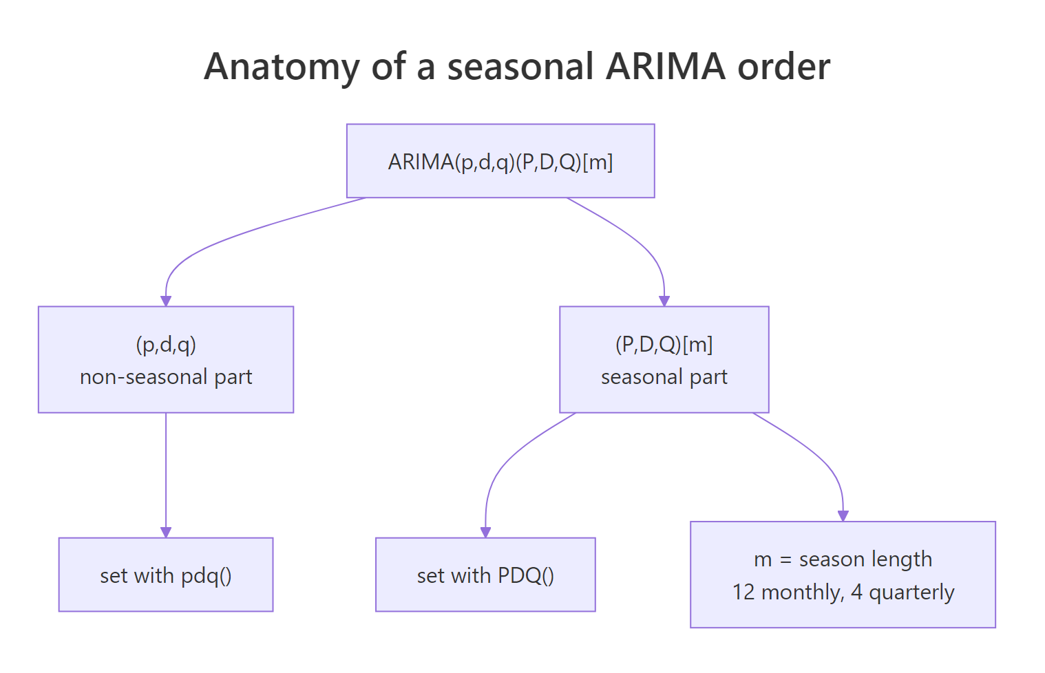
Figure 1: How the (p,d,q)(P,D,Q)[m] order splits into pdq() and PDQ().
The lowercase (p,d,q) is the non-seasonal part: short-term autoregressive terms, differencing, and moving-average terms. The uppercase (P,D,Q) is the same three ideas but one season apart, and [m] is the season length (12 for monthly, 4 for quarterly). You will set these with the pdq() and PDQ() helpers in a moment.
The airline series swings wider as its level rises, and a log transform steadies those swings. You add it right inside the formula: ARIMA(log(value)). fable remembers the transform and undoes it automatically when it forecasts.
fit <- air |> model(auto = ARIMA(log(value)))
report(fit)
#> Series: value
#> Model: ARIMA(2,0,0)(0,1,1)[12] w/ drift
#> Transformation: log(value)
#>
#> Coefficients:
#>          ar1     ar2     sma1  constant
#>       0.5754  0.2614  -0.5553    0.0193
#> s.e.  0.0843  0.0842   0.0771    0.0015
#>
#> sigma^2 estimated as 0.001323:  log likelihood=249.65
#> AIC=-489.29   AICc=-488.82   BIC=-474.88
On the log scale the search lands on ARIMA(2,0,0)(0,1,1)[12] w/ drift, and its AICc of -488.82 is lower (better) than the raw model. The w/ drift on the label means the model adds a constant term, so its forecasts keep climbing the way the passenger counts do instead of flattening out. We will treat this as our working model and call it fit for the rest of the tutorial.
Try it: You can also hand ARIMA() a specific set of orders instead of letting it search. Fit a model with a non-seasonal AR term and a seasonal MA term using pdq(1,1,0) + PDQ(0,1,1), then read the label.
ex_spec <- air |> model(m = ARIMA(log(value)))   # try ~ pdq(1,1,0) + PDQ(0,1,1)
ex_spec
Click to reveal solution
air |> model(m = ARIMA(log(value) ~ pdq(1,1,0) + PDQ(0,1,1))) |> report()
#> Series: value
#> Model: ARIMA(1,1,0)(0,1,1)[12]
#> Transformation: log(value)
#>
#> Coefficients:
#>           ar1     sma1
#>       -0.3395  -0.5619
#> s.e.   0.0822   0.0748
#>
#> sigma^2 estimated as 0.001391:  log likelihood=243.74
#> AIC=-481.49   AICc=-481.3   BIC=-472.86
Explanation: Putting pdq(1,1,0) + PDQ(0,1,1) on the right of the ~ fixes the orders instead of searching. The label confirms it: ARIMA(1,1,0)(0,1,1)[12].
How do you set the seasonal orders yourself and read the model?
When you have a model in mind, the pdq() and PDQ() specials let you spell it out. The most famous seasonal ARIMA is the airline model, ARIMA(0,1,1)(0,1,1)[12]: one ordinary difference, one seasonal difference, and a moving-average term in each part. You write it by putting both helpers on the right of the ~.
fit_manual <- air |> model(manual = ARIMA(log(value) ~ pdq(0,1,1) + PDQ(0,1,1)))
report(fit_manual)
#> Series: value
#> Model: ARIMA(0,1,1)(0,1,1)[12]
#> Transformation: log(value)
#>
#> Coefficients:
#>           ma1     sma1
#>       -0.4018  -0.5569
#> s.e.   0.0896   0.0731
#>
#> sigma^2 estimated as 0.001371:  log likelihood=244.7
#> AIC=-483.4   AICc=-483.21   BIC=-474.77
To prove fable is not doing anything mysterious, here is the exact same model fit with base R's own arima() function. No fable, no tsibble, just the raw engine.
The coefficients match to the last digit: ma1 is -0.4018 and sma1 is -0.5569 in both, and the AIC is -483.4 either way. fable is a tidy front end over the same estimation. Now let's read a fitted model without eyeballing the printout. The tidy() verb returns one row per coefficient as a clean table.
tidy(fit)
#>   .model term     estimate std.error statistic  p.value
#>   <chr>  <chr>       <dbl>     <dbl>     <dbl>    <dbl>
#> 1 auto   ar1        0.575    0.0843       6.83 2.83e-10
#> 2 auto   ar2        0.261    0.0842       3.11 2.33e- 3
#> 3 auto   sma1      -0.555    0.0771      -7.21 3.99e-11
#> 4 auto   constant   0.0193   0.00149     13.0  2.07e-25
Every p.value is tiny, which means each term is doing real work in the model. When you want the model's summary numbers instead of its coefficients, glance() gives you one row of fit statistics.
glance(fit) |> select(.model, sigma2, log_lik, AICc, BIC)
#>   .model  sigma2 log_lik  AICc   BIC
#>   <chr>    <dbl>   <dbl> <dbl> <dbl>
#> 1 auto 0.00132 250. -489. -475.Try it: Compare the automatic model against the hand-built airline model by their AICc. Stack the two glance() rows together and see which is lower.
ex_glance <- glance(fit) |> select(.model, AICc)   # add fit_manual to compare
ex_glance
Click to reveal solution
bind_rows(
  glance(fit)        |> select(.model, AICc),
  glance(fit_manual) |> select(.model, AICc)
)
#>   .model  AICc
#>   <chr>  <dbl>
#> 1 auto   -489.
#> 2 manual -483.
Explanation: The automatic model (auto, AICc -489) edges out the hand-built airline model (manual, AICc -483), so the search found a slightly better fit than the textbook default.
How do you check the model's residuals?
A model is only trustworthy if what it leaves behind, the residuals, looks like random noise. If any pattern is left in the residuals, the model missed something. In fable, augment() adds the fitted values and residuals back onto your data. The .innov column holds the innovation residuals, which are the ones you test.
augment(fit) |> select(index, value, .fitted, .innov) |> head(5)
#> # A tsibble: 5 x 4 [1M]
#>      index value .fitted  .innov
#>      <mth> <dbl>   <dbl>   <dbl>
#> 1 1949 Jan   112    111. 0.00460
#> 2 1949 Feb   118    117. 0.00465
#> 3 1949 Mar   132    131. 0.00476
#> 4 1949 Apr   129    128. 0.00474
#> 5 1949 May   121    120. 0.00468
The .fitted values sit right next to the real value, so you can see the model is tracking the series closely. To test the residuals formally, the Ljung-Box test asks whether any autocorrelation (correlation of the residuals with their own earlier values) is left over. A high p-value is good news: it means you cannot detect leftover pattern.
augment(fit) |> features(.innov, ljung_box, lag = 24, dof = 4)
#>   .model lb_stat lb_pvalue
#>   <chr>    <dbl>     <dbl>
#> 1 auto      29.0    0.0868
The p-value of 0.087 is above 0.05, so the residuals pass: there is no significant autocorrelation left, and the model has captured the structure. The same test exists in base R as Box.test(), which you can run right here on the forecast-package fit from earlier.
Here the p-value is 0.037, just below 0.05. That is expected: fit_f is the raw-scale model from the top of the page, and its residuals still hold a little seasonal autocorrelation. The log-scale fable model above passed the same test at 0.087, which is one more reason to prefer it.
Try it: The p-value depends on how many lags you test. Re-run the base R test with lag = 12 instead of 24 and see how the result changes.
Click to reveal solution
Explanation: At 12 lags the p-value is 0.53, comfortably above 0.05. Testing fewer lags looks only at shorter-term autocorrelation, where this raw model looks clean; the lower p-value back at 24 lags came from the longer-range seasonal pattern it leaves behind.
How do you forecast future values?
Forecasting is one verb: forecast() with a horizon h. Because the series is monthly, h = 24 means two years ahead. fable returns a fable object, which carries a full probability distribution for each future month in the value column, plus the point forecast in .mean.
fc <- fit |> forecast(h = 24)
fc
#> # A fable: 24 x 4 [1M]
#> # Key:     .model [1]
#>    .model    index             value .mean
#>    <chr>     <mth>            <dist> <dbl>
#>  1 auto   1961 Jan t(N(6.1, 0.0013))  453.
#>  2 auto   1961 Feb t(N(6.1, 0.0018))  430.
#>  3 auto   1961 Mar t(N(6.2, 0.0022))  486.
#>  4 auto   1961 Apr t(N(6.2, 0.0025))  502.
#>  5 auto   1961 May t(N(6.3, 0.0028))  522.
#>  6 auto   1961 Jun  t(N(6.4, 0.003))  600.
The .mean column already reads in passenger counts (453, 430, and so on), not log units, because fable undid the log transform for you. The value column shows each forecast as a transformed normal distribution, t(N(...)). To turn a distribution into a plain prediction interval, pipe it through hilo().
fc |> hilo(level = 95) |> select(index, .mean, `95%`) |> head(4)
#>      index .mean                  `95%`
#>      <mth> <dbl>                 <hilo>
#> 1 1961 Jan  453. [421.2056, 485.7503]95
#> 2 1961 Feb  430. [395.6490, 466.3885]95
#> 3 1961 Mar  486. [443.0038, 532.9857]95
#> 4 1961 Apr 502. [454.5652, 553.9548]95The forecast package can forecast too, and its forecast() returns point predictions you can run right now. Here are the first six months from the base fit.
Try it: A 95 percent interval is wide; an 80 percent interval is tighter. Forecast one year ahead (h = 12) and read the 80 percent interval instead.
ex_fc <- fit |> forecast(h = 24)   # change level to 80, then run
ex_fc |> hilo(level = 95) |> nrow()
Click to reveal solution
fit |> forecast(h = 12) |> hilo(level = 80) |> select(index, .mean, `80%`) |> head(3)
#>      index .mean                  `80%`
#>      <mth> <dbl>                 <hilo>
#> 1 1961 Jan  453. [431.7281, 473.9112]80
#> 2 1961 Feb  430. [407.0742, 453.2985]80
#> 3 1961 Mar  486. [457.4106, 516.1986]80
Explanation: The 80 percent interval (432 to 474 in January) is narrower than the 95 percent one (421 to 486). A lower confidence level buys you a tighter range at the cost of catching the truth less often.
How do you compare several SARIMA models at once?
This is where fable pulls ahead of the classic workflow. You can list several models inside one model() call, and fable fits them all and stores each in its own column. Here we fit the automatic model, the hand-built airline model, and a simple seasonal naive baseline that just repeats last year's value.
fits <- air |> model(
  auto   = ARIMA(log(value)),
  manual = ARIMA(log(value) ~ pdq(0,1,1) + PDQ(0,1,1)),
  snaive = SNAIVE(value)
)
glance(fits) |> select(.model, AICc, BIC)
#>   .model  AICc   BIC
#>   <chr>  <dbl> <dbl>
#> 1 auto   -489. -475.
#> 2 manual -483. -475.
#> 3 snaive   NA    NA
The seasonal naive model has no AICc because it estimates no parameters. To compare all three on equal footing, accuracy() reports error measures like RMSE (average size of the errors) and MAPE (average error as a percent).
accuracy(fits) |> select(.model, .type, RMSE, MAE, MAPE)
#>   .model .type     RMSE   MAE  MAPE
#>   <chr>  <chr>    <dbl> <dbl> <dbl>
#> 1 auto   Training  9.93  6.99  2.53
#> 2 manual Training 10.2   7.36  2.62
#> 3 snaive Training 36.3  32.0  11.2
The automatic model has the smallest errors: a MAPE of 2.53 percent, against 11.2 percent for the naive baseline. Fitting and ranking three seasonal ARIMA candidates took a single pipeline.
Try it: Rank the three fitted models from best to worst by their MAPE using arrange().
ex_fits <- fits   # already includes snaive; run accuracy() on it
nrow(accuracy(ex_fits))
Click to reveal solution
accuracy(fits) |> select(.model, MAPE) |> arrange(MAPE)
#>   .model  MAPE
#>   <chr>  <dbl>
#> 1 auto    2.53
#> 2 manual  2.62
#> 3 snaive 11.2
Explanation: arrange(MAPE) sorts ascending, so the smallest error is on top. The automatic model wins, the airline model is a close second, and the naive baseline trails far behind.
Complete Example: forecast air passengers end to end
Here is the whole workflow in one place: convert the data to a tsibble, fit an automatic seasonal ARIMA on the log scale, check the report, and forecast a year ahead with intervals. This is the pattern you will reuse for any seasonal series.
air_ce <- as_tsibble(AirPassengers)
fit_ce <- air_ce |> model(sarima = ARIMA(log(value)))
report(fit_ce)
#> Series: value
#> Model: ARIMA(2,0,0)(0,1,1)[12] w/ drift
#> Transformation: log(value)
#>
#> Coefficients:
#>          ar1     ar2     sma1  constant
#>       0.5754  0.2614  -0.5553    0.0193
#> s.e.  0.0843  0.0842   0.0771    0.0015
#>
#> sigma^2 estimated as 0.001323:  log likelihood=249.65
#> AIC=-489.29   AICc=-488.82   BIC=-474.88
fit_ce |> forecast(h = 12) |> hilo(level = 95) |> select(index, .mean, `95%`) |> head(3)
#> index .mean `95%`
#> <mth> <dbl> <hilo>
#> 1 1961 Jan 453. [421.2056, 485.7503]95
#> 2 1961 Feb 430. [395.6490, 466.3885]95
#> 3 1961 Mar 486. [443.0038, 532.9857]95The forecast for January 1961 is about 453 passengers, with 95 percent confidence that the true value falls between 421 and 486. That is a complete, defensible seasonal ARIMA forecast in five lines of tidy code.
Practice Exercises
These build on the whole tutorial. Each runs in your own R session with fable, tsibble, and feasts loaded. Try each before opening the solution.
Exercise 1: Forecast the quarterly UKgas series
Convert the built-in UKgas series to a tsibble, fit an automatic seasonal ARIMA on the log scale, print the report, and forecast the next 8 quarters. Notice that the season length becomes 4 on its own.
# Convert UKgas to a tsibble, fit ARIMA(log(value)), report, forecast h = 8.
gas <- as_tsibble(UKgas)
# your code here
Click to reveal solution
gas <- as_tsibble(UKgas)
gas_fit <- gas |> model(sarima = ARIMA(log(value)))
report(gas_fit)
#> Series: value
#> Model: ARIMA(0,0,0)(1,1,0)[4] w/ drift
#> Transformation: log(value)
#>
#> Coefficients:
#>          sar1  constant
#>       -0.1938    0.0786
#> s.e.   0.0966    0.0102
#>
#> sigma^2 estimated as 0.01096:  log likelihood=88.05
#> AIC=-170.1   AICc=-169.86   BIC=-162.17
gas_fit |> forecast(h = 8) |> as_tibble() |> select(index, .mean) |> head(4)
#> index .mean
#> <qtr> <dbl>
#> 1 1987 Q1 1249.
#> 2 1987 Q2 649.
#> 3 1987 Q3 363.
#> 4 1987 Q4 853.Explanation: The label [4] confirms fable read the quarterly season automatically. The forecast climbs every Q1 (winter heating) and dips every Q3, exactly the seasonal shape in the data.
Exercise 2: Pick the better model with AICc
Fit two models to air: the automatic one, ARIMA(log(value)), and the airline model, ARIMA(log(value) ~ pdq(0,1,1) + PDQ(0,1,1)). Put both in one model() call, then use glance() and arrange() to rank them by AICc.
# Fit auto and airline in one model() call, then arrange by AICc.
Click to reveal solution
cap_fits <- air |> model(
  auto     = ARIMA(log(value)),
  airline  = ARIMA(log(value) ~ pdq(0,1,1) + PDQ(0,1,1))
)
glance(cap_fits) |> select(.model, AICc) |> arrange(AICc)
#>   .model   AICc
#>   <chr>   <dbl>
#> 1 auto    -489.
#> 2 airline -483.
Explanation: The automatic search wins by AICc (-489 against -483). One model() call fit both, and arrange(AICc) put the better model on top.
Exercise 3: Test the forecast on held-out data
AICc measures fit on the training data. The tougher test is forecasting data the model never saw. Keep every month before January 1959 as training, fit the automatic model, forecast 24 months, and score it against the real values with accuracy().
# Filter index < yearmonth("1959 Jan") for training, fit, forecast h = 24, score with accuracy(., air).
Click to reveal solution
train <- air |> filter(index < yearmonth("1959 Jan"))
cap_fc <- train |> model(auto = ARIMA(log(value))) |> forecast(h = 24)
accuracy(cap_fc, air) |> select(.model, .type, RMSE, MAPE)
#>   .model .type  RMSE  MAPE
#>   <chr>  <chr> <dbl> <dbl>
#> 1 auto   Test   14.6  2.40
Explanation: On the 24 held-out months the model is off by 2.40 percent (MAPE) on average. Test error is the honest measure of how a forecast will behave on the future you actually care about.
Frequently Asked Questions
Should I use fable or the forecast package for seasonal ARIMA? Both fit the same models. Reach for fable when you want a tidy pipeline, tidy output, and the ability to fit and compare many models at once. Reach for the forecast package when you want something lighter that runs anywhere. The SARIMA in R tutorial covers the forecast-package path in full.
Do I always need to write PDQ() in the formula? No. If you leave the right side of ARIMA() blank, it searches both the non-seasonal and seasonal orders for you. You only write pdq() and PDQ() when you want to fix specific orders. One catch: to force a non-seasonal fit you must write PDQ(0, 0, 0), because simply leaving PDQ() out still lets the search add seasonal terms.
Why fit on the log scale with ARIMA(log(value))? When a series swings wider as its level rises (like airline passengers), a log transform makes the swings roughly constant, which suits ARIMA's assumptions. fable remembers the transform and undoes it when forecasting, so your forecasts and intervals come back in the original units.
What does the [12] or [4] in the model label mean? It is the season length, the number of steps in one full cycle. Monthly data has [12], quarterly data has [4], and daily data with a weekly cycle has [7]. fable reads it from the tsibble's interval, so you rarely set it by hand.
When should I trust the automatic model over one I choose myself? Compare them with AICc on the same data, and confirm the winner's residuals pass the Ljung-Box test. If the automatic model has a lower AICc and clean residuals, it is usually the safer choice. A model you pick by hand is worth keeping only when it matches known structure in the series and scores about as well.
Summary
Fitting a seasonal ARIMA in fable is one tidy pipeline from data to forecast. The table below maps each step to its verb.
| Step | fable verb | What it does |
|---|---|---|
| Prepare data | as_tsibble() |
Turns a series into a time-aware data frame |
| Fit | model(ARIMA(value)) |
Searches for or fits a seasonal ARIMA |
| Set orders | pdq() and PDQ() |
Fix the non-seasonal and seasonal parts |
| Read | report(), tidy(), glance() |
Print the model, coefficients, and fit stats |
| Check | augment(), ljung_box |
Test that residuals are random noise |
| Forecast | forecast(h), hilo() |
Predict ahead with prediction intervals |
| Compare | glance(), accuracy() |
Rank several models at once |
The diagram below shows how those steps connect, from a raw series all the way to a forecast.
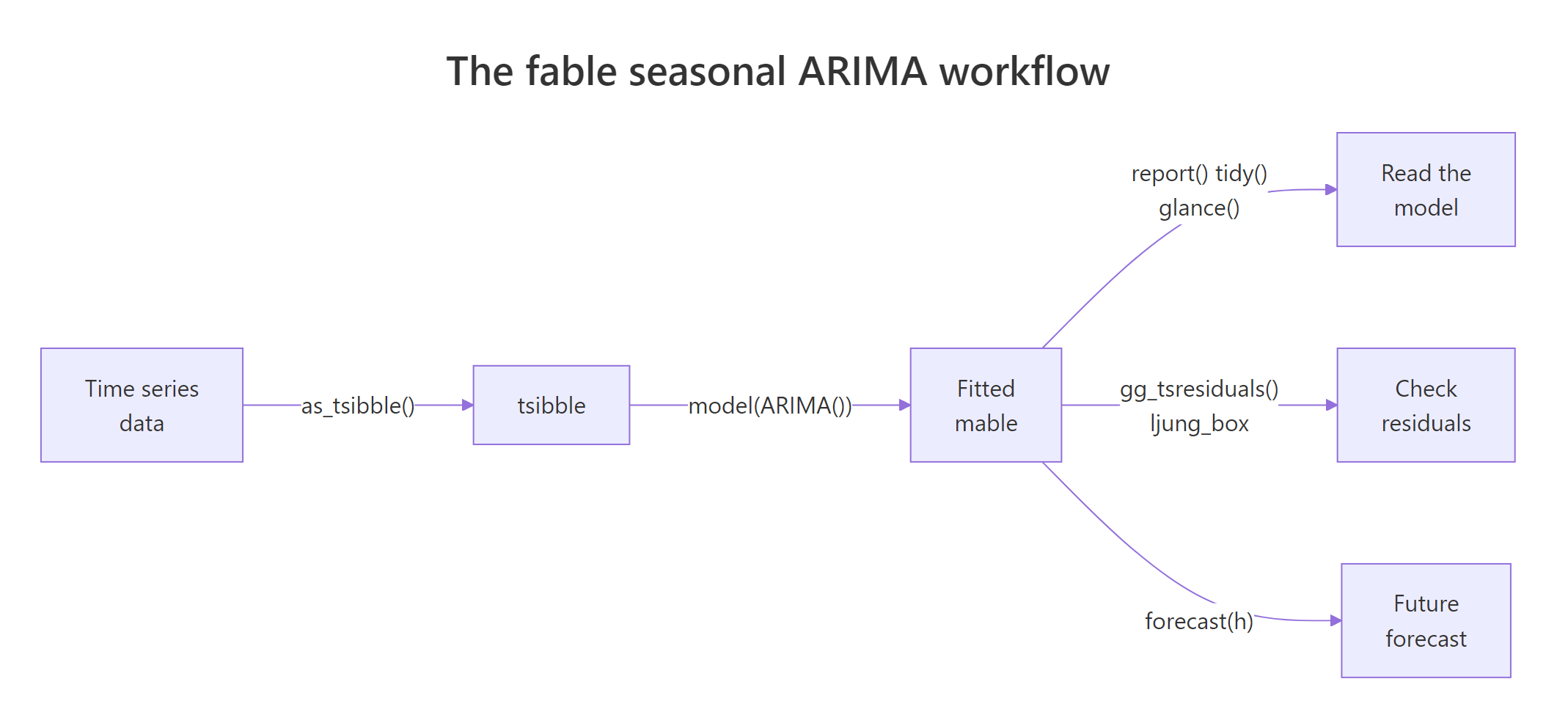
Figure 2: The fable seasonal ARIMA workflow, from tsibble to forecast.
The one idea to carry away: fable does not change the seasonal ARIMA math, it changes the workflow around it. Tidy data goes in, tidy verbs read and check the model, and comparing many candidates is a single call rather than a pile of separate objects.
References
- Hyndman, R.J., & Athanasopoulos, G. - Forecasting: Principles and Practice, 3rd ed. Section 9.9: Seasonal ARIMA models. Link
- Hyndman, R.J., & Athanasopoulos, G. - Forecasting: Principles and Practice, 3rd ed. Section 9.7: ARIMA modelling in fable. Link
- fable documentation - ARIMA() model reference. Link
- tsibble documentation - Reference and vignettes. Link
- feasts documentation - Feature extraction and diagnostics. Link
- R Core Team -
arima()in the stats package. Link
Continue Learning
- SARIMA in R: How to Fit Seasonal ARIMA Models - the same seasonal ARIMA model fit with the forecast package, with the theory of the seasonal orders in depth.
- auto.arima() in R - how automatic order selection searches for the best ARIMA, which is what fable's ARIMA() does under the hood.
- ARIMA Diagnostics in R - a fuller guide to residual checks, the Ljung-Box test, and reading diagnostic plots.