Moving Averages in R: Simple, Weighted, and Exponential
A moving average smooths a time series by replacing each point with the average of a small window of nearby values, so the underlying trend shows through the noise. This guide builds the three kinds you will actually meet, simple, weighted and exponential, from scratch in R, and shows when to reach for each.
What is a moving average, and why smooth a time series?
Real-world measurements wobble. Daily sales, river levels and sensor readings all jump from one step to the next, and those jumps hide the slower story underneath. A moving average is the simplest fix: slide a fixed-size window along the series and replace each point with the mean of the values inside that window. Here is the idea on ten noisy sales figures, smoothed with a three-point window.
The raw sales column zig-zags between 9 and 20. The sma3 column is calmer: each smoothed value is the average of three neighbouring points, so single spikes get diluted. The rollmean() function from the zoo package did the sliding for us, and fill = NA marks the two ends where a full three-point window does not fit.
Nothing magic happened. To prove it, compute the second smoothed value by hand: it is just the mean of the first three sales.
That matches sma3[2] exactly. A moving average is only ever this: pick a window size, average the values inside, then slide the window forward one step and repeat.
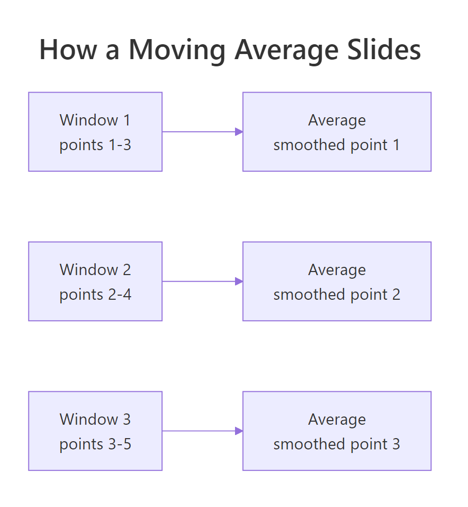
Figure 1: A moving average slides a fixed window along the series, averaging each window into one smoothed point.
Written as a formula, a simple moving average with window size $k$ is
$$\text{SMA}_t = \frac{x_{t-k+1} + x_{t-k+2} + \dots + x_t}{k}$$
where $x_t$ is the value at time $t$ and $k$ is how many points you average. If formulas are not your thing, skip it: the arithmetic in the code above is the whole idea.
Try it: Smooth this short series with a 4-point trailing simple moving average and round the result to two decimals.
Click to reveal solution
Explanation: align = "right" tells rollmean() to end each window at the current point, so the first full 4-point window covers positions 1 to 4. The first three values are NA because a full window does not exist yet.
How do you compute a simple moving average in R?
You just met rollmean(), but base R can do the same job, and one detail matters a lot: where the window sits relative to the point it produces. Let's cover both.
Base R ships stats::filter(), which multiplies each window by a set of coefficients. Give it k copies of 1/k and sides = 2 (a window centred on each point), and you get the same simple moving average.
These are the same numbers as the very first block. Two tools, one result, which is reassuring: the moving average is a fixed recipe, not a package-specific trick.
dplyr, its row-filtering filter() hides the time-series stats::filter(), and you get a confusing error. Write stats::filter() in full whenever you mean the moving-average version.The word "centred" above is the detail that matters. A window can sit in three places relative to the point it fills: ending at it (trailing, align = "right"), centred on it (align = "center"), or starting at it (align = "left"). Trailing and centred are the two you will use, and they answer different questions.
The two columns hold identical numbers, just shifted by one row. The trailing average only ever looks backward, so it is what you use for real-time monitoring and forecasting. The centred average sits symmetrically over each point, which lines the smoothed line up with the raw data, so it is what you use to reveal a trend. Because centred windows need points on both sides, they leave gaps at both ends; trailing windows only leave a gap at the start.
Centred smoothing shines on data with a repeating cycle. The built-in AirPassengers series counts monthly airline passengers from 1949 to 1960, and it climbs every year while swinging up and down within each year. A 12-month centred average spans exactly one year, so the seasonal swings cancel and the underlying growth trend is left behind.
The passengers column bounces between 112 and 148 in the first year, but the trend column barely moves, creeping from 126.7 to 128.8. That is the yearly cycle averaged away, leaving only the slow rise. A picture makes it obvious, so let's plot the raw series with its trend on top.
The grey line is the jagged monthly count; the purple line is the smooth trend the moving average pulled out. This trend line is exactly the first ingredient in classical time series decomposition, so a moving average is not just a chart cosmetic, it is a modelling building block.
data.table::frollmean() computes the same trailing average far faster.Try it: Compute a 6-month trailing simple moving average of AirPassengers and read off the smoothed values for months 6 through 8.
Click to reveal solution
Explanation: With k = 6 and align = "right", the first complete window ends at month 6, so months 1 through 5 are NA and month 6 is the first real value.
What is a weighted moving average, and when is it better?
A simple moving average treats every point in the window as equally important. Often that is wrong: in sales, prices or demand, what happened yesterday usually tells you more than what happened a week ago. A weighted moving average fixes this by giving each position in the window its own weight, with the most recent point counting the most.
The usual choice is linear weights: 1 for the oldest point in the window, 2 for the next, up to $k$ for the newest, all divided by their total so they add up to 1.
$$\text{WMA}_t = w_1 x_{t-k+1} + w_2 x_{t-k+2} + \dots + w_k x_t, \qquad \sum_{i=1}^{k} w_i = 1$$
Let's compute one window by hand first. For a three-point window the weights are 1, 2 and 3 over 6, and we apply them to the first three sales figures.
The newest of the three points, sales[3] = 9, gets weight 3/6, so the answer of 10.17 is pulled toward that recent dip, lower than the simple average of 10.33 you saw earlier. That is the whole point of weighting: recent moves show up faster. Now slide those weights along the entire series with rollapply(), which hands each window to a function of your choice.
Each row is the weighted sum of the three most recent sales, with the newest weighted heaviest. Compare row 4: the simple average was 11.67, but the weighted average is 12.00 because it leans on the recent jump to 14. The weighted line hugs the latest data more tightly than the simple line does.
(1:k)/sum(1:k), keeps the average on the same scale as the series.Try it: Build a 4-point weighted moving average of ex_series where the newest point counts four times as much as the oldest.
Click to reveal solution
Explanation: The weights (1:4)/sum(1:4) are 0.1, 0.2, 0.3 and 0.4. Multiplying each window by these and summing gives an average that leans hardest on the most recent value.
What is an exponential moving average (EMA)?
A weighted moving average uses only the last $k$ points, and gives no weight at all to anything before that window. An exponential moving average takes the idea further: it keeps a running estimate that blends today's value with everything that came before, so old data fades away smoothly instead of being cut off.
The recipe is a single line you apply over and over. Each new average is a blend of the new value and the previous average, controlled by one number, the smoothing factor $\alpha$ (alpha), between 0 and 1.
$$\text{EMA}_t = \alpha\, x_t + (1 - \alpha)\,\text{EMA}_{t-1}$$
Where:
- $x_t$ = the new value at time $t$
- $\text{EMA}_{t-1}$ = the previous average (yesterday's estimate)
- $\alpha$ = the smoothing factor; larger means more weight on the newest value, so a faster reaction
The clearest way to see this is to build it with a loop, seeding the first average with the first data point.
Read the second value: 0.5 * 12 + 0.5 * 10 = 11. The third: 0.5 * 9 + 0.5 * 11 = 10. Every step is half the new point plus half of where you already were. With alpha = 0.5 the average reacts quickly; a smaller alpha would weight past values more heavily and move more slowly.
Loops are fine, but R has a tidier way. Reduce() carries a running result forward through a vector, which is exactly the EMA pattern, and accumulate = TRUE keeps every intermediate value.
Identical to the loop, in one expression. Use whichever reads more clearly to you.
One question remains: how do you pick $\alpha$? In finance and forecasting people usually think in terms of a span $n$, roughly "how many points of memory I want", and convert it with $\alpha = 2/(n+1)$. A 5-point span, for example, gives an alpha of one third.
Try it: Apply an EMA with alpha = 0.5 to the vector c(2, 4, 6, 8), seeding with the first value.
Click to reveal solution
Explanation: Seeded at 2, each step averages the new value with the running total: 0.5*4 + 0.5*2 = 3, then 0.5*6 + 0.5*3 = 4.5, then 0.5*8 + 0.5*4.5 = 6.25.
How do simple, weighted and exponential moving averages compare?
You now have all three. They differ in exactly one way: how much weight each point inside the window carries. A simple average spreads weight evenly, a weighted average ramps it up linearly toward the newest point, and an exponential average lets it decay smoothly so even the oldest points keep a small, non-zero weight.
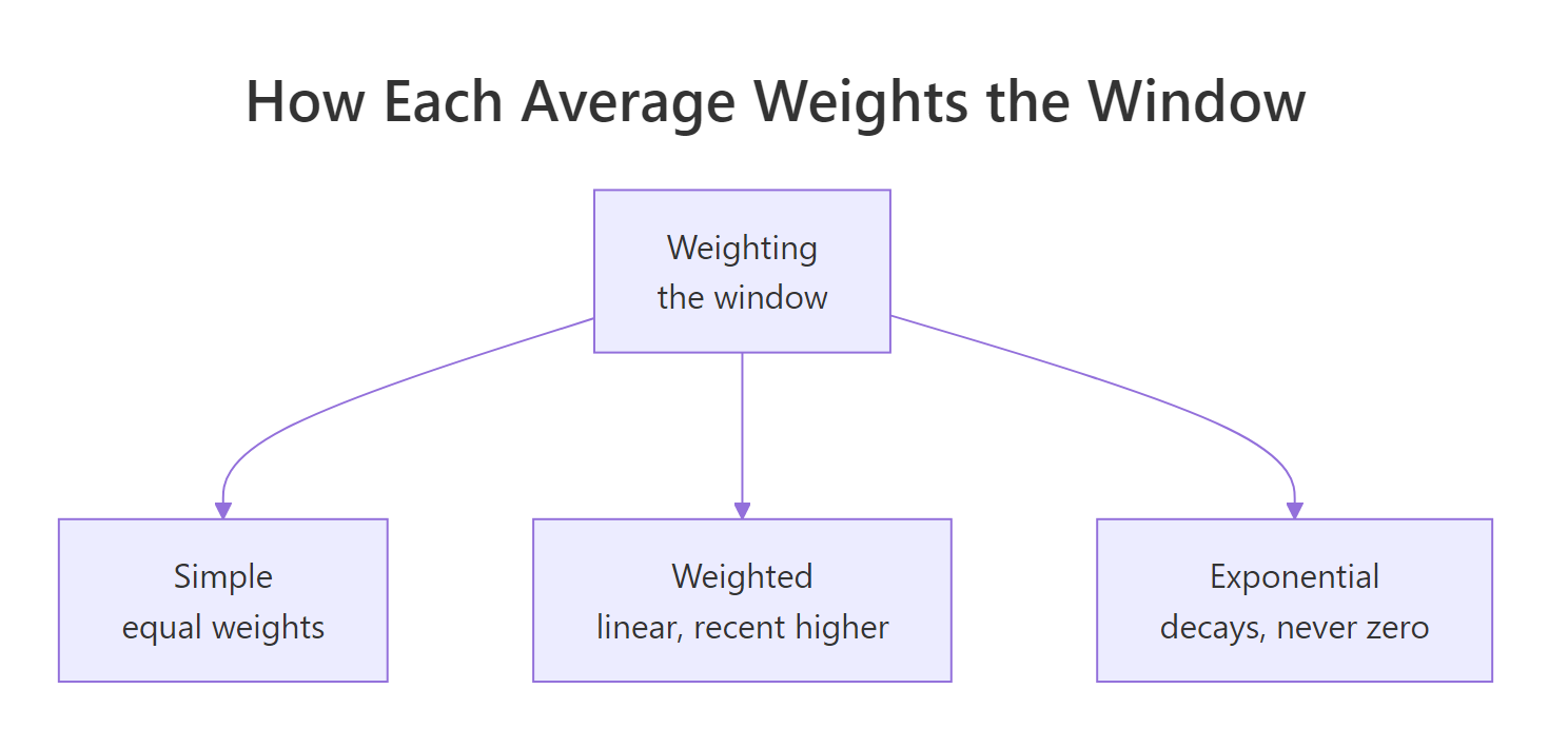
Figure 2: The three averages differ only in how they weight points inside the window.
Put them next to each other on the sales series and the difference in responsiveness shows up in the numbers.
Notice two things. The EMA has values in rows 1 and 2 where the others are NA, because it never waits for a full window, it starts from the first point. And when sales jump, the weighted and exponential columns move toward the new level a step ahead of the simple column. Here is the same comparison as a reference table.
| Average | Weights across the window | Reacts to change | Best for |
|---|---|---|---|
| Simple (SMA) | Equal | Slowest | A steady trend that is easy to explain |
| Weighted (WMA) | Rise linearly to the newest | Medium | When recent points matter but memory is finite |
| Exponential (EMA) | Decay smoothly, never zero | Fastest | Streaming data that needs a quick response |
The one knob you always tune is the amount of smoothing: the window size $k$ for simple and weighted averages, or the smoothing factor $\alpha$ for the exponential one. There is no free lunch here.
Try it: This series repeats every 7 steps. Smooth out the weekly cycle with a centred window that spans one full period.
Click to reveal solution
Explanation: A window of 7, the length of the cycle, averages one full period at every point, so the weekly ups and downs cancel and only the gentle drift (around 20 to 21) survives. The first three and last three positions are NA because a centred 7-window needs three points on each side. Matching the window to the seasonal period is the standard trick for exposing a trend.
How do you forecast with a moving average?
Smoothing looks backward, but you can also use a moving average to guess the next value. The simplest forecast is a flat one: predict that the next observation will equal the average of the last few. Because a forecast can only use data you already have, you must use a trailing (backward-looking) window.
The last three sales were 18, 15 and 20, so the moving-average forecast for the next period is their mean, 17.67. To forecast several steps ahead with this simple method, you just repeat that same number, since you have no new data to update it with.
A flat moving-average forecast is a baseline, not a finished model, because it ignores trend and seasonality. The exponential moving average is the seed of a better family: add trend and seasonal terms to it and you get exponential smoothing (ETS), and a different lens gives you ARIMA. Both are covered in the forecasting tutorials linked at the end.
Try it: Make a 3-step-ahead flat forecast for this series using the mean of its last three values.
Click to reveal solution
Explanation: The last three values are 48, 55 and 60, averaging to 54.33. With no new information arriving, the flat forecast repeats that number for every future step.
Complete example: smoothing and forecasting the Nile
Let's put all three averages to work on a fresh dataset. The built-in Nile series records the annual flow of the river Nile from 1871 to 1970, and it is noisy with a gentle downward shift, a good test for smoothing. We compute a 5-year simple, weighted and exponential average in one place.
Look at 1877, when flow crashed to 813. The centred simple average barely notices (1146.6, because it also averages in the high neighbours on both sides), while the trailing weighted and exponential averages drop hard (1037.9 and 1032.8) because they weight that recent low heavily. Plotting all three against the raw flow makes the difference in how they respond clear.
Finally, a one-step-ahead flat forecast for 1971 is just the mean of the last 5 observed years.
That single number, 767.4, is the plainest possible forecast. It sets the baseline that any real forecasting model has to beat.
Practice Exercises
These combine several ideas from the tutorial. Try each before opening the solution.
Exercise 1: SMA versus EMA on a price series
Compute a 4-point trailing simple moving average and a matching exponential moving average (span 4, so alpha = 2/(4+1)) on the price series below, then compare their final values. Which one sits closer to the latest price of 115?
Click to reveal solution
Explanation: Both land near 112, but the EMA (111.879) tracks the recent climb a touch more tightly because its weights favour the newest prices. On a faster-moving series the gap would be larger.
Exercise 2: a moving-average crossover
A classic trading signal is the "golden cross", where a short-window average rises above a long-window average. Compute a 3-point and a 6-point trailing simple moving average of my_series, then find the first index where the short average crosses above the long one.
Click to reveal solution
Explanation: signal is positive when the short average is above the long one. Comparing each value with the one before it (prev) finds the moment the signal turns from non-positive to positive, which happens at index 10, just as the series recovers from its dip.
Exercise 3: one function, three averages
Write a single function moving_average(x, k, type) that returns a simple, weighted, or exponential moving average depending on type. Test it on the sales vector from the top of the tutorial.
Click to reveal solution
Explanation: match.arg() lets the caller pass just "simple", "weighted" or "exponential" and picks the matching branch. Each branch reuses the exact code from the tutorial, so one function now covers all three averages.
Frequently asked questions
Is a moving average the same as a rolling average?
Yes. "Rolling average", "running average" and "moving average" all name the same idea: a mean taken over a window that slides along the series. R packages tend to use the "roll" spelling, as in rollmean() and rollapply().
Should I use a centred or a trailing moving average?
Use a centred average when you want to see a trend, because it lines up symmetrically with the data. Use a trailing average when the value must be available in real time or you plan to forecast, because it never looks into the future.
How do I choose the window size or smoothing factor?
Start from the structure of your data. If it has a repeating cycle, set the window to one full period. Otherwise pick the smallest window (or largest alpha) that still calms the noise, since more smoothing always adds more lag.
Can a moving average predict future values?
It can give a simple baseline forecast: the mean of the last few points, repeated forward. It ignores trend and seasonality, so treat it as the number a real model like exponential smoothing or ARIMA has to beat.
Summary
A moving average smooths a series by averaging a sliding window; the three types differ only in how they weight the points inside that window.
| Method | R call | One-line idea |
|---|---|---|
| Simple (SMA) | rollmean(x, k) |
plain mean of the last k points, equal weights |
| Weighted (WMA) | rollapply(x, k, weighted sum) |
linear weights, recent points count more |
| Exponential (EMA) | Reduce() or stats::filter() |
recursive blend, weights shrink but never reach zero |
Key things to carry away:
- Use a centred average to reveal a trend and a trailing average to forecast; never forecast with a centred window.
- Match the window to the cycle: a window equal to the seasonal period averages the season away.
- More smoothing means more lag, so pick the smallest window or largest alpha that still calms the noise enough.
fill = NAmarks the edges where a full window does not fit; centred windows leave gaps at both ends.
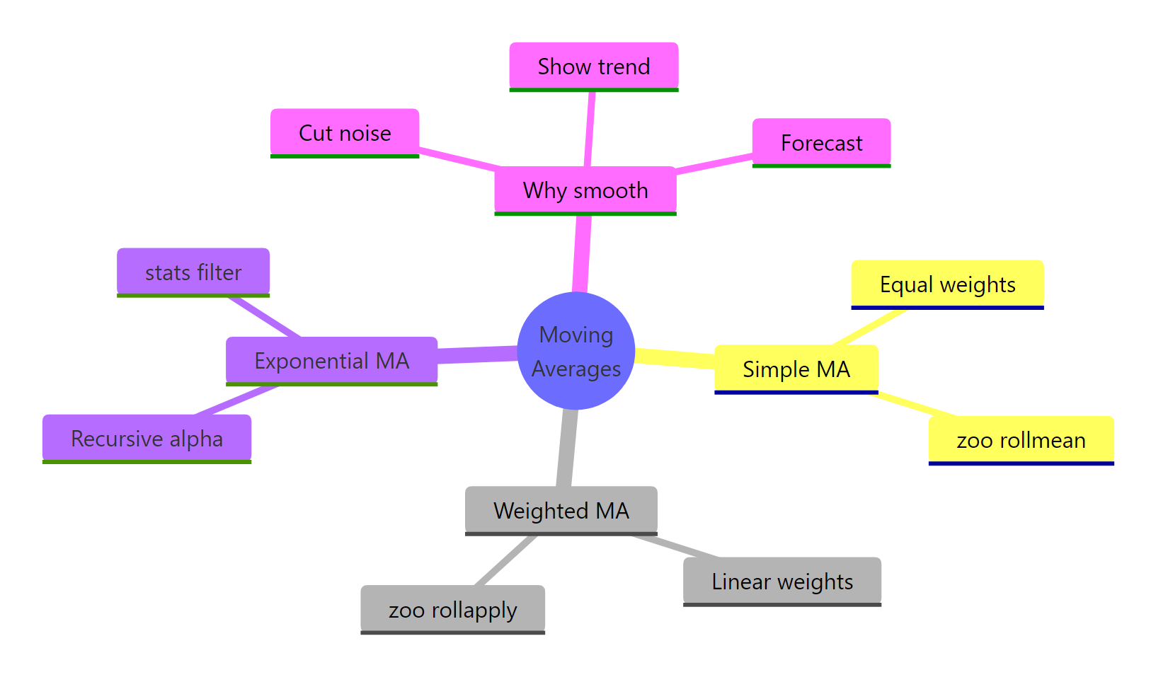
Figure 3: The moving-average toolkit at a glance: three methods, three uses.
References
- Hyndman, R.J. & Athanasopoulos, G. - Forecasting: Principles and Practice (3rd ed.), Moving Averages. Link
- Hyndman, R.J. & Athanasopoulos, G. - Forecasting: Principles and Practice (3rd ed.), Classical Decomposition. Link
- zoo package on CRAN - rolling window functions including
rollmeanandrollapply. Link - zoo reference -
rollmean()documentation. Link - R stats reference -
filter()for linear filtering of time series. Link - Wikipedia - Moving average (simple, weighted and exponential definitions). Link
- NIST/SEMATECH e-Handbook of Statistical Methods - EWMA control charts. Link
Continue Learning
- Time Series Decomposition in R: STL vs Classical - the moving-average trend you built here is the first step of classical decomposition.
- Test Stationarity in R: ADF, KPSS, and Differencing - after smoothing out a trend, check whether what remains is stationary enough to model.
- Time Series Objects in R: ts, xts, zoo, or tsibble? - understand the
tsandzooobjects that these moving-average functions consume and return.