Hierarchical and Grouped Time Series in R: Reconciliation
A hierarchical time series is a set of series that must add up: store sales sum to region sales, region sales sum to national sales. Forecast each series on its own and those totals stop matching. Reconciliation fixes that by nudging every forecast by the smallest amount that makes the whole set add up again.
What is a hierarchical time series?
Australia's tourism board publishes quarterly overnight trips for every state. Add the eight state numbers together and you get the national number, exactly, in every quarter of the record. That word "exactly" is the whole subject of this tutorial. Let's pull the real data first and look at it. Everything here uses the tidyverts stack: tsibble holds the data, fable fits the models.
The tourism dataset ships inside the tsibble package. It is quarterly, it runs from 1998 to 2017, and it is broken down by region, state and trip purpose. We only want state-level totals for now, so we add up the regions and purposes inside each state and each quarter.
Read the header before the rows. A tsibble: 640 x 3 [1Q] says we have 640 rows, three columns and a quarterly index. Key: State [8] says the rows are not one series, they are eight separate series stacked on top of each other, told apart by the State column. A tsibble always needs an index (the time column) and a key (whatever identifies each individual series). We converted to a plain tibble first because summarise() behaves differently on a tsibble, then converted back once the totals were computed. The .by = argument is dplyr's inline grouping: it says "give me one sum for each distinct combination of Quarter and State", and does the same job as wrapping the call in group_by().
Eighty quarters times eight states gives exactly the 640 rows we see. That is the raw material. Trips counts overnight trips in thousands, so 551. means about 551,000 trips.
This shape, many small series that roll up into bigger ones, is what a hierarchy looks like.
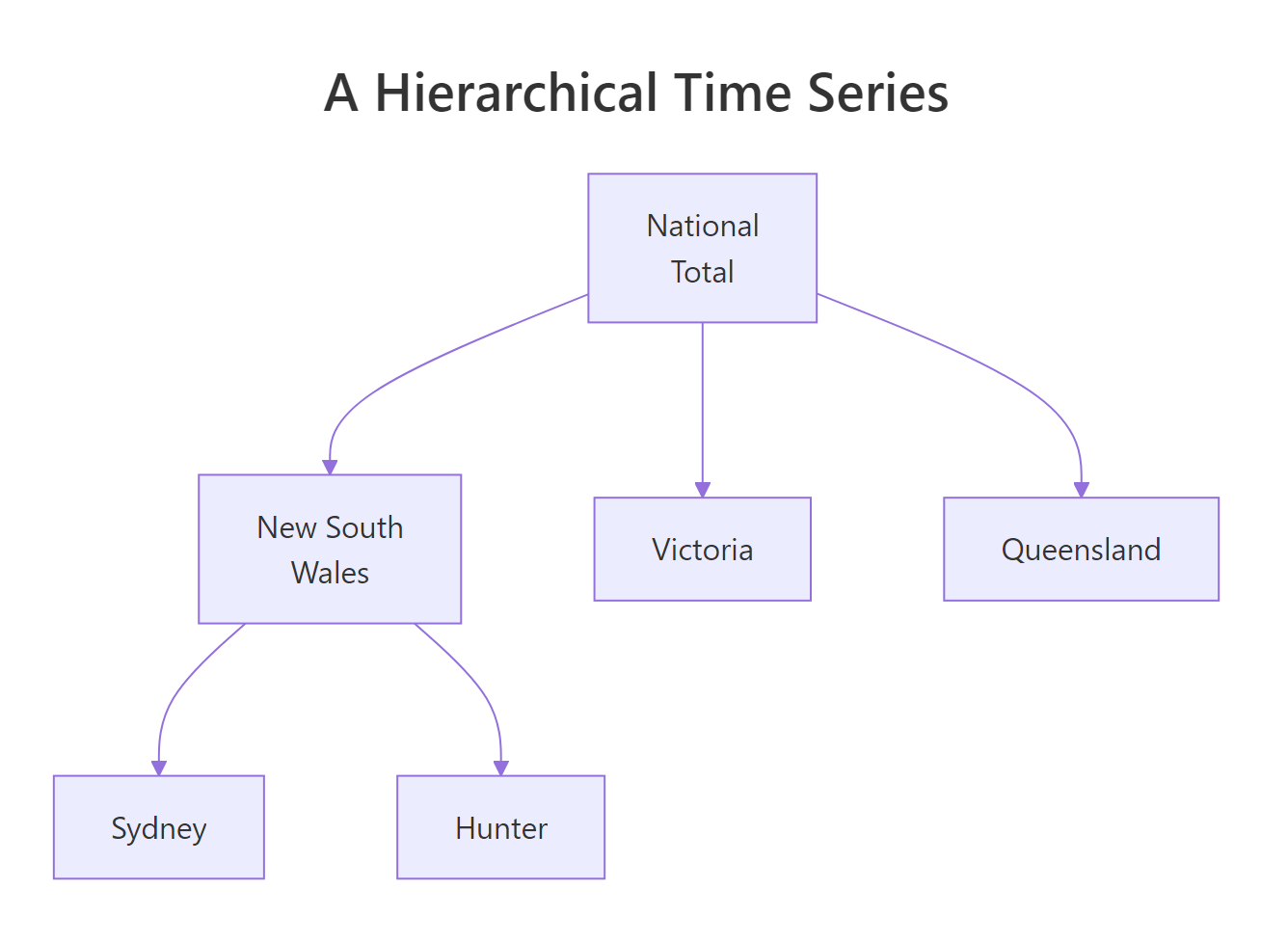
Figure 1: A hierarchy: every level is the sum of the level below it.
The bottom of the tree holds the finest series you actually measure. Every level above it is a sum of the level below. The single series at the very top is usually the one your CEO cares about, and the ones at the bottom are the ones your operations team cares about.
Now let's verify the claim about adding up. Take a single quarter, print all eight states and add them together.
yearquarter("2017 Q4") turns the text into the same quarterly type that the index uses, so the comparison works. The filter leaves eight rows, one per state, and sum() adds their Trips column.
Australians took about 27.6 million domestic overnight trips in the last quarter of 2017. That number is not an estimate or an approximation. It is the sum of the eight rows above it, and it will be the sum of those eight rows in every single quarter of the data.
Try it: Work out what share of the 2017 Q4 national total each state accounts for, and print the three biggest.
Click to reveal solution
Explanation: as_tibble() drops the tsibble machinery so sum(Trips) runs over all eight rows instead of being blocked by the key. Three states carry more than three quarters of Australian domestic tourism, which is worth remembering: hierarchies are usually very lopsided.
Why don't independent forecasts add up?
The obvious way to forecast a hierarchy is to forecast each piece separately. Fit a model to the national series, fit a model to each state series, publish all nine numbers. That approach fails in a specific way, and seeing it happen once is the fastest route to understanding why reconciliation exists.
The reason it fails is that the national model never looks at the states. It sees one series of numbers and finds the trend and seasonality in that series. Each state model does the same for its own series. Nothing in that process knows the nine forecasts are supposed to be related.
Let's build the national series, fit exponential smoothing to everything, forecast a year ahead, and compare the national forecast with the sum of the state forecasts. ETS() is fable's exponential smoothing model, which picks its own trend and seasonal form automatically.
Follow the pipeline. model(ETS(Trips)) fits one model per series, so it produces one model for national and eight for trips. forecast(h = 4) extends each of them four quarters past the end of the data. The .mean column holds the point forecast. We then pull out the national point forecasts, collapse the state point forecasts into one sum per quarter, join those two tables on Quarter, and take the difference.
The gap column is the damage. In 2018 Q4 the national model predicts 28,627 thousand trips while the eight state models add up to 27,166 thousand. Roughly 1.46 million trips exist in one forecast and not in the other. There is no way to publish both numbers and have them both be true.
A forecast set with gaps like this is called incoherent. A forecast set where every total equals the sum of its parts is called coherent.
Notice also that the gap grows with the horizon: 144 in the first quarter, 1,461 in the fourth. Forecast errors accumulate independently in each model, so the further out you look, the larger the difference between the two sets of numbers.
Try it: The raw gap is hard to judge without context. Express it as a percentage of the national forecast instead.
Click to reveal solution
Explanation: A half-percent disagreement in the first quarter is easy to hand-wave away. A five-percent disagreement a year out is a different conversation entirely, and it is the one you will be having with whoever owns the budget.
How do you build a hierarchy with aggregate_key()?
To fix incoherence, fable first has to know that the eight state series belong to one hierarchy. Right now trips is just eight unrelated series that happen to sit in the same table. The function that adds the structure is aggregate_key().
aggregate_key() takes a key specification and an aggregation rule, and returns a new tsibble containing the original series plus every total implied by that structure. Ask for State and you get the eight states back, plus a ninth series holding their sum.
Three things changed. The row count went from 640 to 720, which is the 80 extra rows of the new national series. Key: State [9] confirms there are now nine series instead of eight. And the State column prints as <chr*> rather than <chr>, because it is no longer plain text.
The rows shown are the new series. Its State value is the special marker <aggregated>, which is how fable says "this row is a total across every state, not one particular state". The Trips value of 23,182 for 1998 Q1 is the sum of all eight states in that quarter, computed by the Trips = sum(Trips) rule we passed in.
Printing the distinct keys makes the whole structure visible at once.
One total plus eight states. That is the complete hierarchy fable will now reason about, and the <aggregated> row is the only thing we added.
<chr*> means. It mostly behaves like text, but to filter on it you use the helper is_aggregated() rather than comparing against a string, and to turn it back into ordinary text you call as.character().Try it: Use is_aggregated() to pull out only the national rows and count them.
Click to reveal solution
Explanation: Eighty quarters, one national row each. Flip the test to !is_aggregated(State) and you get the other 640 rows, the eight original state series.
How do you reconcile forecasts with fable?
Now for the part that fixes the gap. Reconciliation is a step that sits between fitting models and producing forecasts. You fit your models as usual, then you tell fable "take these fitted models and produce a coherent version of their forecasts using this method". The verb is reconcile().

Figure 2: Reconciliation maps base forecasts down to a bottom level with G, then sums them back up with S.
The forecasts you get before reconciliation have a name: base forecasts. They are the raw, independent, incoherent predictions from each model. Reconciliation never refits anything. It takes the base forecasts as input and adjusts them.
Here we fit one ETS model per series, then add three reconciled versions of it side by side so we can compare them later. Keeping the unreconciled base column is deliberate.
Two method names appear in the code below, so here is what each does in plain words before you run it. bottom_up(base) keeps the eight state forecasts exactly as they are and replaces the national forecast with their sum. min_trace(base, method = ...) adjusts all nine forecasts at once, picking the adjustments that make the reconciled forecast errors as small as possible; "ols" and "mint_shrink" are two different assumptions about those errors, and the next section derives both from scratch.
The result is a mable, a table of fitted models with one row per series and one column per model specification. The base column holds the ETS fits. The three new columns are not new fits, they are the same fits tagged with a reconciliation rule, which is why the model descriptions are identical across every column.
Those descriptions are worth a glance. ETS(M,A,N) for ACT means multiplicative errors, an additive trend and no seasonality. ETS(A,A,A) for the national total means additive everything including seasonality. Each series got the model that suited it, chosen automatically.
Now forecast all four specifications at once and lay the first quarter out side by side. pivot_wider() from tidyr turns the four model rows per state into four columns.
Read down each column. The bu column is identical to base for all eight states and differs only in the last row, because bottom-up keeps the state forecasts exactly as they are and replaces the total with their sum. The ols and mint columns nudge every single number, states included, and land on a slightly different total.
That is the essential difference. Bottom-up discards one forecast and trusts eight. The min_trace methods keep information from all nine and spread the correction across all of them.
Do the numbers actually add up now? Let's check rather than assume.
For each method we pick out the national forecast with is_aggregated(State) and the sum of the eight state forecasts with its negation, then compare. The base row disagrees with itself by 144. The other three rows match to the decimal.
That equality is not a coincidence and not a rounding artefact. Every reconciliation method in fable is constructed so the constraint holds exactly, for every quarter of the horizon.
Try it: Coherence should hold at every horizon, not just the first. Check the last quarter.
Click to reveal solution
Explanation: The base gap has grown to 1,460 while all three reconciled methods still match exactly. Note how far apart the reconciled totals are from each other though: 27,166 against 28,464. Coherence guarantees the numbers are consistent, not that different methods agree.
What is the summing matrix, and what does reconciliation actually compute?
If you only want to use reconciliation, the previous section is enough and you can skip to the next one. This section opens the box, because understanding the two matrices makes every method name in fable obvious instead of arbitrary.
Every reconciliation method, without exception, is the same two steps:
- Take the base forecasts for all series and produce an estimate of the bottom-level series only.
- Sum those bottom-level estimates back up to fill in every other level.
Step 2 is mechanical and identical for every method. Step 1 is where methods differ. Let's build both steps by hand on a hierarchy small enough to print, then confirm our hand calculation matches what fable produced.
Our mini hierarchy is three states, so four series in total: one national plus ACT, the Northern Territory and Tasmania. We forecast one quarter ahead and collect the four base forecasts into a plain named vector.
We pulled the .mean column out as a bare numeric vector, labelled it with the series names, reordered it so the total comes first, and shortened the labels so the matrices below stay readable. This vector is what the maths calls $\hat{y}$, the base forecasts.
Sanity check the incoherence: 700.7 plus 263.2 plus 1120.2 is 2084.1, but the total forecast says 2052.3. Off by 31.8.
The summing matrix, written $S$, is the object that encodes "which series add up to which". It has one row per series in the hierarchy and one column per bottom-level series. Each row says how to build that series out of the bottom ones.
diag(3) makes a 3x3 identity matrix and rbind() stacks a row of ones on top of it. Read the result one row at a time. The Total row is all ones, meaning the total is one of each bottom series added together. The ACT row is 1 0 0, meaning ACT is just ACT. The identity block at the bottom is always there, because every bottom series is trivially equal to itself.
So if $b$ is a vector of the three bottom-level values, then $Sb$ is the full vector of all four series. That is all $S$ does, and it never changes for a given hierarchy.
The mapping matrix, written $G$, does step 1: it turns the four base forecasts into three bottom-level estimates. Different choices of $G$ are different reconciliation methods. Put them together and you get the one equation that describes every method in this tutorial:
$$\tilde{y}_h = S G \hat{y}_h$$
Where:
- $\hat{y}_h$ = the base forecasts, $h$ steps ahead, one per series (our
yhat, length 4) - $G$ = the mapping matrix that produces bottom-level estimates (3 rows by 4 columns)
- $S$ = the summing matrix that rebuilds every level (4 rows by 3 columns)
- $\tilde{y}_h$ = the reconciled, coherent forecasts (length 4)
Because the result always comes out of $S$, it is coherent automatically. Coherence is built into the shape of the calculation, which is why it holds exactly rather than approximately.
Bottom-up is the simplest possible $G$: ignore the total, keep the three state forecasts.
cbind() glues a column of zeros onto the left of a 3x3 identity matrix, and %*% is R's matrix multiplication operator (a plain * would multiply element by element, which is not what we want here). The first column of G_bu is all zeros, which is the matrix way of saying "throw the national forecast away". The identity block copies the three state forecasts through untouched. Then S %*% bottom_bu sums them back up.
The three state numbers came out unchanged, and the total became 2084.1, exactly their sum. Bottom-up in one line of matrix algebra.
The problem with bottom-up is that first column of zeros. The national model saw eighty quarters of a smooth, high-volume series, which is usually the easiest thing in the hierarchy to forecast well, and that column of zeros discards its forecast completely.
Minimum trace reconciliation, or MinT, chooses $G$ to minimise the total variance of the reconciled forecast errors. The name is literal: those variances sit on the diagonal of the error covariance matrix, and the trace of a matrix is the sum of its diagonal entries, so minimising the trace is minimising the total error variance. The solution has a closed form:
$$G = (S' W_h^{-1} S)^{-1} S' W_h^{-1}$$
Where:
- $W_h$ = the covariance matrix of the base forecast errors, $h$ steps ahead
- $S'$ = the transpose of the summing matrix
- $(\cdot)^{-1}$ = matrix inverse
Nobody knows $W_h$ exactly, so every practical method is a different guess at it, and that guess is exactly what the method argument of min_trace() selects. The simplest guess is that all errors are equally sized and uncorrelated, $W_h = kI$, where $I$ is the identity matrix and $k$ is any positive number (it cancels out of the formula). That is method = "ols", and it collapses the formula to $G = (S'S)^{-1}S'$, which we can compute directly.
solve() inverts a matrix and t() transposes one, so this is the formula copied straight across. Look at the ACT row of G_ols: it takes a quarter of the national forecast, three quarters of the ACT forecast, and subtracts a quarter of each other state. Every bottom estimate is a blend of all four base forecasts, with the weights falling out of the hierarchy's shape.
The reconciled numbers are 2060.2, 692.8, 255.2 and 1112.2, and the three states now add to the total: 692.8 plus 255.2 plus 1112.2 is 2060.2. Two matrices we built by hand did the entire job, and they are the same two min_trace(base, method = "ols") builds internally.
Do not expect these figures to match the ols column of the earlier eight-state table. They should not: $S$ and $G$ are built from whichever hierarchy you hand them, so a three-state hierarchy produces different weights, and therefore different adjustments, from an eight-state one.
Try it: Build the summing matrix for a hierarchy with four bottom series instead of three.
Click to reveal solution
Explanation: Five rows because the hierarchy has five series (one total plus four bottom), four columns because four of them are at the bottom. In general $S$ is always n by m, where n counts every series and m counts the bottom ones.
When should you use bottom-up, top-down, or middle-out?
Three older methods predate MinT and still show up constantly in forecasting teams, so it is worth knowing exactly what each one does and where it breaks.
Bottom-up forecasts only the bottom-level series and adds them up. It preserves every bottom-level forecast perfectly and needs no extra assumptions. Its weakness is noise: individual stores or regions are often erratic, and adding up eight noisy forecasts gives you a noisy total, even though the total itself was smooth and easy to forecast.
Top-down does the opposite. It forecasts only the top series, then splits that number down using historical proportions. Let's watch it on the mini hierarchy.
Look at the last row: the top-down total is 2052, identical to the base total. Every state forecast moved down slightly to fit under that ceiling. forecast_proportions decides the split using each state's own forecast share rather than its historical average, which handles states whose share is trending.
That preserved total is top-down's defining property, and also its ceiling. If the national model was wrong, top-down cannot fix it, because it never consults the state models at all. It is guaranteed to be no better than the top forecast it starts from.
Middle-out picks a level in between, forecasts that, then goes bottom-up above it and top-down below it. It suits deep hierarchies where one middle level, say region, has the cleanest data. In fable it is middle_out().
Here is the comparison in one place.
| Method | What it uses | What it discards | Pick it when |
|---|---|---|---|
bottom_up() |
Bottom-level forecasts only | Every model above the bottom | Bottom series are clean and plentiful |
top_down() |
Top-level forecast plus proportions | Every model below the top | Bottom series are sparse, intermittent or brand new |
middle_out() |
One chosen middle level | Models above and below that level | A middle level has the best data quality |
min_trace() |
Every forecast in the hierarchy | Nothing | Almost always, if you have residuals |
min_trace() is the modern default because it is the only one of the four that uses all the information. Its method argument picks the guess at $W_h$, and the choice matters less than people expect.
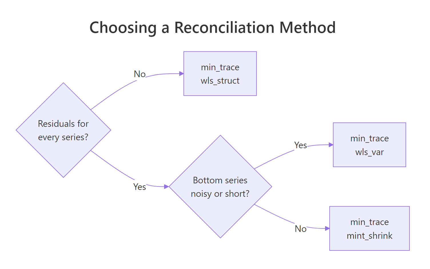
Figure 3: Which min_trace method to reach for first.
method |
Assumption about errors | Notes |
|---|---|---|
"ols" |
All equal and uncorrelated | Ignores scale, so big and small series get equal say |
"wls_struct" |
Variance proportional to how many series were summed | Needs no residuals at all |
"wls_var" |
Variance from each model's own residuals | Good default when the series differ a lot in size |
"mint_shrink" |
Full covariance, shrunk towards the diagonal | Usually the best when you have enough history |
Try it: The table above showed that top-down keeps the national number, but not whether the three adjusted state forecasts actually land on it. Check that top-down is coherent too.
Click to reveal solution
Explanation: Coherent, and equal to the original base total of 2052.3. Top-down buys you consistency without touching the number at the top.
How do you handle grouped series that don't nest?
Everything so far assumed a clean tree: each region belongs to exactly one state, each state to exactly one country. Real data often does not have that shape.
Australian tourism is also broken down by trip purpose: business, holiday, visiting friends and relatives, and other. Purpose does not sit under state, and state does not sit under purpose. They cut across each other. Every combination of state and purpose exists, so there are two different routes from the bottom cells up to the same grand total.
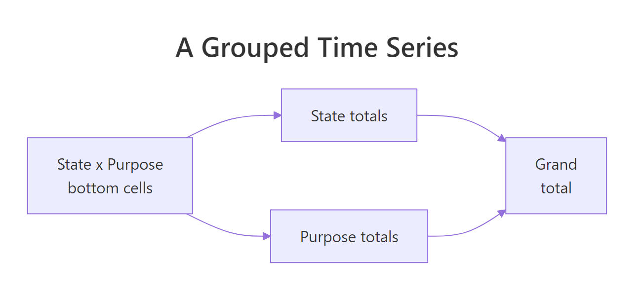
Figure 4: A grouped structure has two routes to the same grand total.
A structure like this is called a grouped time series rather than a hierarchical one. The distinction is exactly this: a hierarchy has one unique path from bottom to top, a grouped structure has several.
In aggregate_key() the operator tells fable which one you mean. Nesting uses a forward slash, State / Region, meaning "regions live inside states". Crossing uses an asterisk, State * Purpose, meaning "these two attributes are independent, give me the totals for both". You can mix them, as in (State / Region) * Purpose.
We will use three states here so the key table prints in full. Dropping the filter() line scales it to all eight without any other change.
Twenty series, and the arithmetic explains every one. Twelve bottom cells (3 states times 4 purposes), plus 3 state totals, plus 4 purpose totals, plus 1 grand total.
The printed rows show how the marker doubles up. Row 1 has <aggregated> in both columns, so it is the grand total. Rows 2 to 4 are aggregated over purpose but not state, so they are state totals. Rows 5 to 8 are the reverse, purpose totals across all three states. The 12 rows hidden below are the bottom cells with a real value in both columns.
Now reconcile it. The code is identical to the hierarchical case, because fable does not care which structure you built.
Each of the four columns computes the grand total a different way: the single grand-total series, the sum of the three state totals, the sum of the four purpose totals, and the sum of the twelve bottom cells. Combining the two is_aggregated() tests with & selects exactly one band of the structure at a time.
All four routes give 22,170. In a grouped structure coherence is a stronger requirement than in a hierarchy, because every path has to land on the same answer, and MinT delivers it.
hts is still on CRAN but is no longer developed, and its authors point new work at fable. One aggregate_key() call covers nested, crossed and mixed structures alike.Try it: Run the same four-way check on the unreconciled base forecasts.
Click to reveal solution
Explanation: Four routes, four different answers, spread across 433 thousand trips. A grouped structure gives incoherence more ways to show up, which is exactly why it needs reconciliation more than a simple hierarchy does.
Does reconciliation actually improve accuracy?
Coherence is worth having on its own, but the interesting question is whether reconciliation also makes the forecasts more accurate. Most tutorials assert that it does and move on. Let's actually measure it.
The test is an ordinary holdout. Train on everything up to the end of 2016, forecast the four quarters of 2017, and compare against what really happened. All four methods are trained on identical data, so any difference is the reconciliation and nothing else.
Nine series times four quarters gives 36 forecasts per method, which is the sanity check that nothing got dropped. Now score them. Crucially, we score each level of the hierarchy separately, because reconciliation affects the top and the bottom in opposite directions and a single blended number would hide that completely.
accuracy() takes the fable and the full dataset, matches forecasts to actuals by date and key, and computes error metrics. RMSE is the root mean squared error in trips; MASE compares the model against a seasonal naive benchmark, where below 1 means better than that benchmark.
At the top of the hierarchy the unreconciled base forecast wins. ols gives up 21 thousand trips of RMSE, about 1.6 percent, and bottom-up gives up 198 thousand, about 15 percent. Bottom-up doing worst here is exactly what the theory predicted: it deleted the national model, which was the best model in the set.
Now the same scoring at the state level, averaged across the eight states.
The order flips. ols is now best at 227, beating base at 239 by 4.7 percent, and it is the only method whose MASE drops below 1, meaning it is the only one beating a seasonal naive forecast on the states.
Look at bu and base: identical to the decimal on both metrics. That is not a bug. Bottom-up leaves every bottom-level forecast exactly as it found it, so at the bottom level it is the base forecast. Its only effect is on the levels above.
ols costs 1.6 percent at the top and pays back 4.7 percent at the bottom, and it makes every number in the set consistent. Whether that trade is good depends on which level your decisions are made at, and the only way to know is to measure it on your own data.The general finding in the research literature is that MinT-family methods usually improve accuracy across a hierarchy taken as a whole, with the gains concentrated in the sparser lower levels. That is what we see here.
Try it: Put a number on what reconciliation bought at the state level.
Click to reveal solution
Explanation: A 4.7 percent RMSE reduction on every state, obtained without fitting a single extra model. The state forecasts improved purely because reconciliation fed information from the national series into them.
Complete Example: an end-to-end hierarchical forecast
Let's put the whole workflow together in the order you would actually run it. Build the hierarchy, fit models, reconcile, forecast, and report the number the business asked for.
We use min_trace(method = "ols") because the holdout test above showed it was the best of the four on this data. On your own data, run that holdout first and let it choose for you.
This time we fit on the complete history including 2017, since the holdout has done its job and there is no reason to withhold real data from the final model. About 29.1 million trips in the first quarter of 2018, easing to 27.5 million in the winter quarter. Every one of these numbers is the exact sum of the eight state forecasts sitting underneath it.
A chart makes the seasonal pattern and the continuation obvious.
We split the data into a grey history layer and a blue forecast layer, then draw both on the same axes. The forecast picks up the upward trend of the last few years and repeats the yearly shape, with the Q1 peak and the Q3 trough carried forward.
The recipe is five steps, and it does not change with the size of the hierarchy:
- Shape the data as a tsibble with an index and a key.
- Call
aggregate_key()to declare the structure,/for nesting and*for crossing. - Fit models with
model(), keeping an unreconciled base column. - Add reconciliations with
reconcile(). - Call
forecast()once and get every method back together.
Practice Exercises
Exercise 1: Build and reconcile a region hierarchy
Tasmania has five tourism regions in the tourism data. Build a hierarchy of those regions with their state total on top, reconcile with mint_shrink, and prove that the reconciled region forecasts for 2018 Q1 add up to the Tasmania forecast while the base ones do not. Save the hierarchy to my_hts.
Click to reveal solution
Explanation: The base row is off by 43 thousand trips, roughly 4 percent of Tasmania's quarterly total. MinT lands between the two base numbers, which is typical: it does not simply trust the total or the parts, it weighs both.
Exercise 2: Bake off four methods on the region hierarchy
Using my_hts from Exercise 1, hold out 2017, forecast it with base, bottom_up, min_trace(ols) and min_trace(mint_shrink), and rank all four by mean RMSE across every series. Save the ranking to my_bakeoff.
Click to reveal solution
Explanation: ols wins again, mint_shrink loses to plain base here, and bottom-up is worst. Six short, noisy series are not enough history for the shrinkage estimator to learn a reliable covariance matrix, which is exactly the situation where the simpler ols or wls_struct methods do better.
Exercise 3: Build a grouped structure from scratch
Build a grouped State * Purpose structure for Tasmania and ACT only, reconcile with min_trace(method = "wls_struct"), and confirm that the grand-total forecast equals the sum of the bottom cells. Work out how many series the structure should contain before you run it. Save it to my_grouped.
Click to reveal solution
Explanation: Fifteen series: 8 bottom cells (2 states times 4 purposes), 2 state totals, 4 purpose totals and 1 grand total. wls_struct is the right pick here because it derives its weights from the structure alone and never touches the residuals, so it works even when some of these small series fit badly.
Frequently Asked Questions
Do I still need the hts package?
No. hts was the original R package for this and it still works, but it is in maintenance mode and its own authors point new work at fable. hts wanted your data as a wide matrix with encoded column names, which is awkward to build and easy to get wrong. aggregate_key() reads the structure off your existing long-format columns instead.
Which min_trace method should I use by default?
Start with "mint_shrink" if you have a reasonable amount of history, since it uses the most information. Use "wls_struct" when series are short, sparse or fit badly, because it needs no residuals at all. Then run the holdout bake-off from the accuracy section and let the data decide. Exercise 2 above is a real case where "ols" beat "mint_shrink".
Can I use ARIMA, or mix different models across the hierarchy?
Yes to both. reconcile() operates on whatever is in the mable, so model(m = ARIMA(Trips)) works identically. You can also fit several model types at once, as in model(ets = ETS(Trips), arima = ARIMA(Trips)), and reconcile each of them separately. Different series can end up with genuinely different fitted models, which is the normal case.
Why did reconciliation make my top-level forecast worse?
Because reconciliation optimises the whole hierarchy, not any single level. If your top series was already the easiest to forecast, spreading information from noisier lower series into it can cost a little accuracy there while gaining more further down. We measured exactly that above. If the top-level number is all that matters to you, forecast it directly and use top-down to fill in below it.
Does reconciliation work on prediction intervals too?
Yes. forecast() returns a distribution in the Trips column, not just a point forecast, and fable reconciles the whole distribution rather than only the mean. Call hilo() on the fable to see the reconciled intervals, and note that reconciled intervals are usually narrower than base intervals at the aggregate levels.
Can reconciliation produce a negative forecast?
Yes, and it is worth checking for. Reconciliation adds and subtracts amounts across series, so a bottom-level series already sitting close to zero, an intermittent product or a tiny region, can be pushed below zero by the adjustment. Nothing in the arithmetic prevents it, because the only thing being enforced is that the numbers add up. Inspect the bottom level of your reconciled forecast for negatives, and if they appear, forecast a transformed series where negatives cannot occur rather than clipping them at zero, since clipping breaks the coherence you just paid for.
What if my hierarchy has thousands of bottom series?
The MinT formula inverts matrices whose size grows with the number of series, so very large hierarchies get slow and memory-hungry. "wls_struct" and "wls_var" use diagonal weight matrices and scale far better than "mint_shrink". Beyond that, common practice is to reconcile within sub-hierarchies, for example one region at a time, rather than solving the whole structure at once.
Summary
The workflow, in the order you run it:
| Step | Function | What it does |
|---|---|---|
| 1 | as_tsibble() |
Declare the time index and the series key |
| 2 | aggregate_key() |
Add every implied total, / nests and * crosses |
| 3 | model() |
Fit one model per series, keep a base column |
| 4 | reconcile() |
Attach one or more reconciliation methods |
| 5 | forecast() |
Produce coherent forecasts for every method at once |
The ideas worth carrying away:
- Coherence is not optional in a business setting. Independent forecasts disagreed by 5 percent a year out on this data, and nothing in R warned us.
- Reconciliation never refits anything. It is a linear adjustment of forecasts you already had, so trying four methods costs almost nothing.
- Every method is $\tilde{y} = SG\hat{y}$. Only $G$ changes; $S$ is fixed by the hierarchy.
- Bottom-up throws away the top model, top-down throws away the bottom ones. MinT uses everything, which is why it is the default worth reaching for.
- Grouped is not hierarchical. When attributes cross rather than nest, use
*and check that every aggregation path agrees. - Measure the trade by level. Reconciliation typically costs a little at the top and pays more at the bottom, and only your own holdout can tell you the balance.
References
- Hyndman, R.J. and Athanasopoulos, G. - Forecasting: Principles and Practice, 3rd edition. Chapter 11.1: Hierarchical and grouped time series. Link
- Hyndman, R.J. and Athanasopoulos, G. - Forecasting: Principles and Practice, 3rd edition. Chapter 11.3: Forecast reconciliation. Link
- fabletools reference -
reconcile(): forecast reconciliation. Link - fabletools reference -
min_trace(): minimum trace forecast reconciliation. Link - fabletools reference -
aggregate_key(): aggregate a dataset over the key variables. Link - Wickramasuriya, S.L., Athanasopoulos, G. and Hyndman, R.J. - Optimal forecast reconciliation for hierarchical and grouped time series through trace minimization. Journal of the American Statistical Association 114(526), 804-819 (2019). Link
- Athanasopoulos, G., Hyndman, R.J., Kourentzes, N. and Panagiotelis, A. - Forecast reconciliation: a review. International Journal of Forecasting 40(2), 430-456 (2024). Link
- Hyndman, R.J. et al. -
hts: Hierarchical and grouped time series. CRAN package page. Link
Continue Learning
- fable in R: Tidy Time Series Forecasting with tsibble - the tsibble and fable foundations this tutorial builds on, including how
model(), mables and fables fit together. - Forecast Accuracy in R: MAE, RMSE, MAPE, and MASE - what the RMSE and MASE numbers in the bake-off actually measure, and which one to trust when they disagree.
- Combining Forecasts in R: Ensemble Averaging - the other way to get more out of models you already fitted, by averaging across models instead of across levels.