Empirical Bayes in R: James-Stein and Shrinkage
Empirical Bayes is a method that estimates a prior from your own data, then uses it to pull each noisy estimate toward the group average. That pull, called shrinkage and made famous by the James-Stein estimator, lowers your total error when you estimate many quantities at once. This guide builds both ideas from scratch in R, using only base R so every number here runs in your browser.
Why do raw averages mislead you on small samples?
Imagine you run a sports desk and you want to predict how well 18 baseball players will hit this season. All you have so far is each player's first 45 at-bats. The obvious move is to use each player's early batting average as your prediction. Let's load that exact situation, the real 1970 data that Bradley Efron and Carl Morris studied, and look at it.
The avg45 column is the raw estimate, and season is the truth we are trying to hit. Right away something looks off. Clemente batted a blistering .400 across 45 at-bats, but his real season average was .346. The raw number overstated his ability.
That is not bad luck for one player, it is a pattern. Let's measure how wide the raw averages spread out, and where their center sits.
The raw averages run from .156 all the way to .400, centered around .265. Here is the key point: 45 at-bats is a tiny sample, so a player at either extreme got there partly on luck. A cold streak of 7-for-45 does not mean a .156 hitter, and a hot 18-for-45 does not mean a .400 hitter. Both extremes will drift back toward the pack.
Try it: Summarize how spread out the 18 raw averages are with a single number. Standard deviation is a natural choice.
Click to reveal solution
Explanation: The raw averages have a standard deviation of about 0.07. A good chunk of that spread is just sampling noise from 45 at-bats, not real talent differences.
What exactly is shrinkage?
If the extremes are inflated by luck, the fix is intuitive: pull every estimate a little toward the group average. A cautious prediction sits between what one player did and what players do on average. That pulling is called shrinkage, and in its simplest form it is just a weighted average.
Let's do it by hand. We will keep a fraction of each player's distance from the group mean and throw the rest away. A factor of 0.5 keeps half the gap.
Clemente's .400 became .333, and Alvis's .156 became .210. Every value moved toward .265, the extremes most of all. The diagram below shows the recipe: take one unit's noisy estimate, take the shared group average, and blend them.
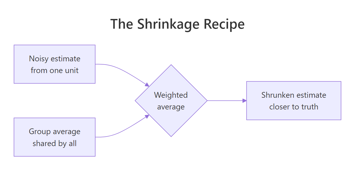
Figure 1: Shrinkage blends one unit's noisy estimate with the shared group average.
Does this cautious blending actually predict the season better? We can check, because we know the true season averages. The standard scorecard is total squared error: add up the squared gap between each prediction and the truth. Smaller is better.
Shrinking cut the total error from 0.0753 to 0.0292, more than halving it. We deliberately biased every prediction toward the middle, and the predictions got better. That trade is the whole game.
Try it: A factor of 0.5 helped. Try shrinking harder with 0.3 (keep only 30 percent of each gap) and see whether the total error falls further.
Click to reveal solution
Explanation: Keeping only 30 percent of each gap drops the error to 0.0223, better still. For this data the true talent differences are small, so heavy shrinkage pays off. The obvious next question is how to pick the factor without peeking at the answer.
How does the James-Stein estimator pick the shrinkage factor?
We chose 0.5 and then 0.3 by hand, but that only worked because we could see the season truth. In real life you cannot. The James-Stein estimator solves this: it reads the right shrinkage factor straight from your data, no peeking required.
Here is the intuition. If your estimates are bunched tightly together, they are mostly noise, so shrink hard. If they are spread far apart, real differences are driving them, so shrink gently. The estimator turns that idea into one formula. For $p$ quantities each measured with noise of variance 1, shrinking toward zero:
$$\hat{\theta}^{JS} = \left(1 - \frac{p-2}{\sum_{i=1}^{p} y_i^2}\right) y$$
Where:
- $y_i$ = the raw measurement for quantity $i$
- $p$ = how many quantities you are estimating at once
- $\sum y_i^2$ = the total squared size of the measurements, which grows when they spread out
The term in parentheses is the shrinkage factor. When the measurements spread out, the denominator grows, the fraction shrinks, and the factor moves toward 1 (gentle shrinkage). If you are not interested in the formula, skip ahead, the code below is all you need.
The famous part is Stein's paradox: as soon as you estimate three or more quantities at once ($p \ge 3$), this shrunken estimator beats the raw measurements on total error, always. Let's watch it happen. We invent 10 true values, observe each with noise, and score both estimators against the truth we secretly know.
The estimator picked a shrinkage factor of 0.404 on its own, and its total error (9.882) came in below the raw error (10.790). One run could be luck, though. Let's repeat the whole experiment 2,000 times and see who wins on average.
Across 2,000 fresh datasets the James-Stein estimator averaged 8.354 total error versus 9.969 for the raw measurements, and it beat the raw estimator in 77 percent of individual runs. Shrinking toward an arbitrary point, zero, with a factor read off the data, reliably beats the obvious estimator.
Try it: The paradox needs at least three quantities. Rerun the single-dataset idea with just 3 means and confirm James-Stein still comes out ahead.
Click to reveal solution
Explanation: Even with only three means, James-Stein (1.818) edges out the raw estimate (2.010). Notice we use $p - 2 = 1$ in the factor. Below three quantities the correction turns off and there is nothing to gain.
Does James-Stein actually help on the real baseball data?
Simulations are convincing, but you came for real data. Let's point James-Stein at the 18 batting averages. We treat each average as a noisy measurement of a player's true skill, shrink toward the group mean instead of zero, and use the version of the formula built for a shared target:
$$\hat{\theta}_i^{JS} = \bar{y} + \left(1 - \frac{(p-3)\,\sigma^2}{\sum_i (y_i - \bar{y})^2}\right)(y_i - \bar{y})$$
Here $\bar{y}$ is the group mean and $\sigma^2$ is the noise variance of a single average. A batting average from 45 at-bats has a known noise variance, roughly $\bar{p}(1-\bar{p}) / 45$, so we can plug everything in.
The estimator chose to keep only 21 percent of each player's gap from the mean, and the payoff is dramatic: total error dropped from 0.0753 to 0.0213, about 3.5 times more accurate than trusting the raw averages. This is the original 1975 Efron-Morris result, and you just reproduced it from scratch.
Try it: js_est holds the James-Stein estimate for every player. Find the worst early hitter and read off his raw, James-Stein, and true averages to see which way he moved.
Click to reveal solution
Explanation: Alvis looked like a .156 hitter after 45 at-bats. James-Stein lifted him to .242, and his real season average was .200. The shrunken guess landed much closer to the truth than the low raw number.
How do you estimate the prior from the data itself?
So far we have shrunk toward the group mean, but we never asked how strong that pull should be in a principled way. Empirical Bayes answers that by treating the whole group as evidence about a prior distribution, then letting Bayes' rule do the shrinking. The word "empirical" means we do not assume a prior, we estimate it from the data.
The workflow has two steps, shown below. First, look at all 18 players together and fit a prior distribution for batting skill. Second, combine that prior with each player's own record to get a posterior estimate.
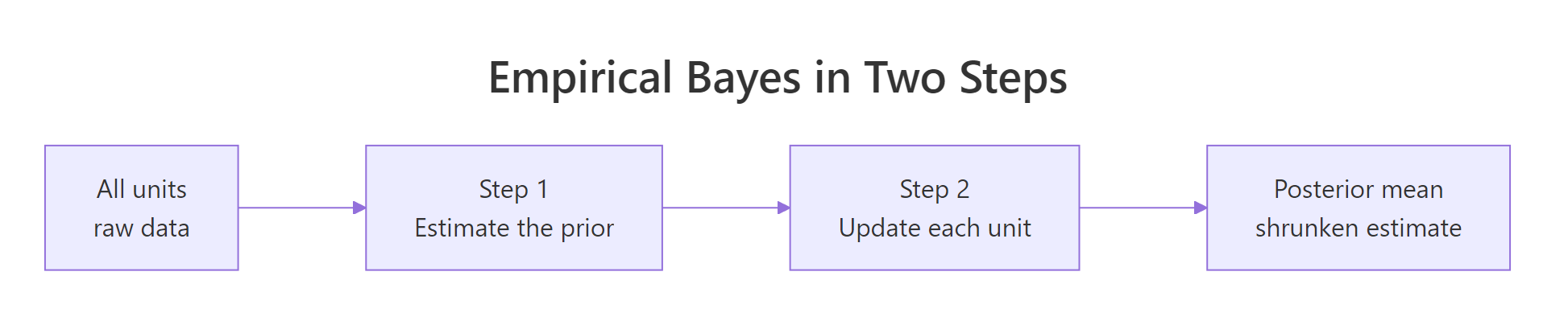
Figure 2: Empirical Bayes estimates the prior from all units, then updates each one.
For batting averages the natural prior is a Beta distribution, because a Beta paired with hit-or-miss counts gives a clean posterior. That pairing is the beta-binomial model, and it is the engine behind conjugate priors. We fit the prior's two shape parameters, $\alpha$ and $\beta$, by maximum likelihood: we find the pair that makes the observed hit counts most probable.
The fitted prior is centered at 0.265, exactly the group average, and its strength is about 795. You can read $\alpha + \beta$ as a number of "pseudo at-bats" the prior is worth. With each player owning only 45 real at-bats, that heavy prior will pull everyone strongly toward the center.
Now the second step. The posterior mean for a Beta prior updated with hits out of at-bats has a simple closed form:
$$\hat{p}_i^{EB} = \frac{x_i + \alpha}{n_i + \alpha + \beta}$$
Where $x_i$ is the player's hits, $n_i$ is the at-bats, and $\alpha, \beta$ come from the fitted prior. You add the prior's pseudo-counts to the real counts and divide. Let's apply it and score it against the season truth.
Empirical Bayes cut the total error to 0.0228, about 3.3 times better than the raw averages, right in line with the James-Stein result. Notice how tight the eb column is: every prediction sits near 0.27. With only 45 at-bats apiece, the data barely distinguishes these players, so leaning on the crowd is the sensible choice.
Try it: Use the fitted prior to score a brand-new player who went 30 hits in 100 at-bats.
Click to reveal solution
Explanation: A raw .300 hitter with 100 at-bats gets shrunk all the way to .269. With 795 pseudo at-bats in the prior, 100 real at-bats simply cannot shift the estimate far.
How much should each estimate shrink, and when does it backfire?
The last example hints at the rule that governs everything: the more data a unit has, the less it gets shrunk. The weight the prior carries is $(\alpha + \beta) / (n + \alpha + \beta)$. When $n$ is tiny the prior dominates, and when $n$ is huge the data wins. Let's watch that weight fall as at-bats climb.
With 10 at-bats the prior gets almost 99 percent of the vote, so the estimate is basically the group mean. By 500 at-bats the prior's weight has dropped to 61 percent, and the player's own record starts to speak for itself. Shrinkage is not a fixed amount, it scales with how much you actually know about each unit.
Try it: A hot hitter is batting .400. Give him 300 at-bats instead of 45 and see how far the prior still pulls him in.
Click to reveal solution
Explanation: Even with 300 at-bats at a .400 clip, empirical Bayes predicts .302. That is a lot of shrinkage, and it points to the method's blind spot.
Shrinkage assumes the units are interchangeable, drawn from one shared prior. When one unit is genuinely special, the crowd-based prior pulls it too far toward the average. Clemente is the cautionary tale: he really was an all-time great, yet the method treated his hot start as mostly luck.
Clemente's true .346 sits far above the shrunken .273. Empirical Bayes pulled him too hard because it assumed he was an ordinary player having a lucky month. On this batch the aggressive shrinkage still lowered total error, but it under-credited the one player who deserved the benefit of the doubt.
Complete Example
Baseball is the classic story, but the real payoff of empirical Bayes is any setting with many units and little data each. Think of 200 products on a store, each with a handful of visits and a few purchases, where you need a trustworthy conversion rate for every one. Raw rates from a dozen visits are hopeless. Here is the full workflow end to end.
The fitted prior recovered shape parameters near the true 8 and 40 we simulated from, and the empirical-Bayes rates were 2.6 times more accurate than the raw rates. Because the trial counts vary here, each product shrinks by a different amount: the ones with only a handful of visits lean almost entirely on the prior, while the well-observed ones keep most of their own signal. That per-unit adaptivity is exactly what you want in production.
Practice Exercises
These combine several ideas from the tutorial. Try each before opening the solution. The variables from earlier code blocks (p_hat, eb_est, season, grand_mean, alpha0, beta0, sigma2) are still available.
Exercise 1: Does the leader change under shrinkage?
Shrinkage moves every estimate, so it could reshuffle the rankings. Find the player with the highest raw average and the player with the highest empirical-Bayes estimate. Are they the same person?
Click to reveal solution
Explanation: Clemente tops both lists. Shrinkage pulls everyone toward the center but preserves the order here, because it shrinks all players by nearly the same amount when their at-bats are equal.
Exercise 2: Which predictor wins overall?
Compare three strategies for predicting the season averages: the raw 45-at-bat averages, predicting the grand mean for everyone, and the empirical-Bayes estimates. Compute each one's total squared error against season.
Click to reveal solution
Explanation: The raw averages (0.0753) are by far the worst. Predicting the grand mean for everyone (0.0243) is already a big improvement, and empirical Bayes (0.0228) edges it out by adapting to each player. When per-unit data is this thin, most of the gain comes from simply pulling toward the center.
Exercise 3: When does the shrinkage weight go negative?
The James-Stein weight from the baseball section was 1 - (p - 3) * sigma2 / S, where S is the spread of the estimates. Write that weight as a function of S for p = 18, then evaluate it at S = 0.02, 0.05, and 0.10. What does a negative weight tell you?
Click to reveal solution
Explanation: When the spread S is small (0.02), the weight goes negative, a signal that the estimates are so bunched they are almost pure noise. In practice you clamp a negative weight to 0, which means shrink all the way to the mean. As S grows, the weight climbs toward keeping more of each estimate.
Frequently Asked Questions
Is estimating the prior from the same data a form of double-counting?
Yes, empirical Bayes uses the data twice: once to fit the shared prior and once to update each unit. That is why it is an approximation to a full Bayesian analysis, not the same thing. It holds up well when you have many units, because any single unit contributes only a little to the prior, so the prior is nearly independent of the estimate it then adjusts. With only a handful of units the approximation gets shaky and the fitted prior can look more certain than it should.
How is empirical Bayes different from full Bayesian inference?
Full Bayes fixes the prior before seeing the data, from theory or belief, and carries the uncertainty about the prior through to the final answer. Empirical Bayes instead estimates the prior's parameters from the data and then treats them as known, which ignores the uncertainty in that estimate. What you get in return is that you never have to invent a prior, and with many units the two approaches land in almost the same place.
Does this only work for batting averages and proportions?
No. The beta-binomial model here fits proportions, but the same recipe (fit one shared prior across all units, then pull each unit toward it) works for other data types. Counts pair with a Gamma-Poisson model, and normal measurements are exactly the James-Stein case from earlier. You pick the prior family that matches your data; the shrinkage logic does not change.
How many units do I need before shrinkage helps?
James-Stein needs at least three quantities before it can beat the raw estimates, which is where Stein's paradox begins. Empirical Bayes needs enough units to pin down the prior: a handful gives a noisy prior, while dozens or hundreds (the 18 players or 200 products here) give a stable one. More units mean a sharper borrowed prior and a better-calibrated pull for every estimate.
Summary
Empirical Bayes and James-Stein are two paths to the same destination: shrink noisy estimates toward a shared center to lower your total error.
| Idea | What it does | Key formula or output |
|---|---|---|
| Raw average | Trusts each small sample fully | Total error 0.0753 on the baseball data |
| Fixed shrinkage | Blends estimate with the group mean by hand | Error fell to 0.0292 at factor 0.5 |
| James-Stein | Reads the shrinkage factor from the data | 3.5 times more accurate on the batting averages |
| Empirical Bayes | Fits a prior from all units, then updates each | 3.3 times more accurate, and handles counts directly |
| Shrinkage weight | Scales with sample size | More data means less shrinkage |
The mental model to keep: an estimate from little data is mostly noise, so lean on the crowd; an estimate from lots of data has earned trust, so let it speak. James-Stein and empirical Bayes just turn that instinct into arithmetic, and they come with a guarantee that the total error goes down. The one caution is exchangeability: shrinkage assumes your units come from one shared population, so a genuinely exceptional unit will be under-credited.
References
- Efron, B. & Morris, C. (1975). Data Analysis Using Stein's Estimator and Its Generalizations. Journal of the American Statistical Association. Link
- James, W. & Stein, C. (1961). Estimation with Quadratic Loss. Proceedings of the Fourth Berkeley Symposium. Link
- Efron, B. & Hastie, T. (2016). Computer Age Statistical Inference, Chapter 7: James-Stein Estimation and Ridge Regression. Cambridge University Press. Link
- Robinson, D. Understanding Empirical Bayes Estimation (Using Baseball Statistics). Variance Explained. Link
- Morris, C. (1983). Parametric Empirical Bayes Inference: Theory and Applications. Journal of the American Statistical Association. Link
- R Core Team. optim: General-purpose Optimization. R Documentation. Link
Continue Learning
- Conjugate Priors in R - The Beta-Binomial machinery behind the empirical-Bayes update step, explained with closed-form posteriors.
- Ridge Regression in R - James-Stein's close cousin, applying the same shrinkage idea to regression coefficients.
- Approximate Bayesian Computation in R - Bayesian inference when you cannot even write down the likelihood.