ABC in R: Bayesian Inference Without a Likelihood
Approximate Bayesian Computation (ABC) is a way to do Bayesian inference when you cannot write down the likelihood. Instead of plugging numbers into a formula, you simulate fake datasets from candidate parameter values and keep the ones whose simulations resemble your real data. The kept values are your posterior. This post builds ABC from scratch in R, verifies it against a posterior we can compute exactly, then applies it to a model that has no likelihood at all. Everything is base R plus one plotting package, and the core sampler is just a few lines.
What does a likelihood do, and why can't you always write one down?
Every Bayesian calculation you have seen rests on one quantity: the likelihood. If you have read the MCMC tutorial, you have already leaned on it heavily. The likelihood is the probability of your observed data for a given setting of the parameters, written $P(\text{data} \mid \theta)$. Bayes' rule then combines it with your prior belief to give the posterior:
$$P(\theta \mid \text{data}) \propto P(\text{data} \mid \theta) \times P(\theta)$$
For a coin, the likelihood is easy. If a coin lands heads with probability $p$, the chance of seeing 32 heads in 50 flips is a binomial formula you can evaluate in one call to dbinom(). MCMC, variational Bayes, and every other standard method need this formula, because they all work by scoring how well each candidate $\theta$ explains the data.
Now picture a model where you cannot write that formula. You can simulate an epidemic spreading through a town, a population's genes drifting over generations, or customers queuing at a call center. Running the model forward is easy: give it parameters, press go, watch data come out. But writing $P(\text{data} \mid \theta)$ would mean summing over every hidden path the process could have taken, and that sum has no closed form. The likelihood exists in principle, yet it is out of reach.
Here is the move that saves us. If you can simulate data from a parameter value, you can check whether that value tends to produce data like what you actually saw. Parameters that keep producing your data are credible; parameters that never do are not. That single idea, replacing "evaluate the likelihood" with "simulate and compare," is Approximate Bayesian Computation. Let us watch it work on the coin, where we can check the answer.
We observed 32 heads in 50 flips and want the coin's bias $p$. Our prior is total ignorance: $p$ is equally likely to be anything between 0 and 1. The code below draws thousands of candidate $p$ values from that prior, simulates 50 flips for each, and keeps only the candidates that produced exactly 32 heads.
Look at what happened. We never wrote a likelihood. We drew 100,000 guesses, threw away every one that did not reproduce our 32 heads, and about 1,947 survived. The average of those survivors is 0.6348. The exact posterior mean for this problem, which we can compute by hand because the coin has a tidy formula, is 0.6346. ABC landed on the right answer using nothing but simulation and a filter.
p that reproduces 32 heads often is, by definition, a value the data support, so the pile of survivors is a sample from the posterior. ABC turns "score the likelihood" into "simulate and sieve."Try it: Change the observed count to 40 heads out of 50 and rerun the sieve. The posterior should shift toward a more biased coin. The exact posterior mean for 40 heads is 41/52.
Click to reveal solution
The posterior mean jumps to about 0.789, matching the exact value 0.7885. More heads means the sieve keeps larger values of p.
How does the ABC rejection algorithm work, step by step?
That one code block hid a four-step loop that has a name: the ABC rejection sampler. It is worth slowing down and naming each step, because everything else in this post is a variation on these four moves.
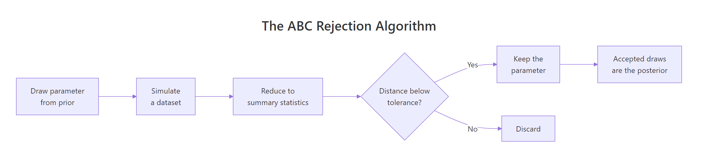
Figure 1: The ABC rejection sampler: draw, simulate, summarise, accept within tolerance.
The four steps are: draw a parameter from the prior, simulate a dataset with it, reduce the simulation to a summary you can compare, and accept the parameter if that summary is close enough to the observed one. For the coin, the summary was simply the number of heads, and "close enough" meant "exactly equal." Let us watch a single trip through the loop so the mechanics are concrete.
This candidate drew p = 0.266, simulated 50 flips, and got 12 heads. We observed 32, so 12 is nowhere near, and this candidate is rejected. A biased-low coin like 0.266 rarely produces 32 heads, which is exactly why the sieve filters it out. Repeat this millions of times and only the plausible values survive.
Now let us package the loop into a reusable function and read off the full posterior it produces, not just the mean. A posterior is a distribution, so we want its spread and a credible interval too.
The function returns the pile of accepted p values, our posterior sample. Its mean is 0.634, its standard deviation is 0.066, and a 95% credible interval runs from 0.505 to 0.757. That interval is the ABC answer to "how sure are we about the coin's bias."
Because this particular problem is a coin with a flat prior, statisticians know the exact posterior: it is a Beta distribution with parameters 33 and 19. We do not need to derive that here; we just use it as an answer key to check ABC against.
The exact posterior has mean 0.635, standard deviation 0.066, and a 95% interval from 0.501 to 0.759. Compare that to the ABC numbers above: they agree to two decimals across the board. ABC is not a rough approximation here, it reproduces the exact posterior. Seeing the two match on a solvable problem is what lets us trust ABC on the unsolvable ones later. A picture makes the agreement obvious.
The purple histogram is the ABC sample; the dark curve is the exact posterior. They sit on top of each other.
Try it: Run the sampler with a much larger N (say 500,000) and confirm the posterior mean barely moves while the number of accepted draws grows. More draws sharpen the estimate without changing where it sits.
Click to reveal solution
With 500,000 candidates, about 9,670 are accepted and the mean settles at 0.635. More simulations buy you a smoother posterior, not a different one.
Why does ABC compare summary statistics instead of raw data?
For the coin we compared head counts, not the exact sequence of heads and tails. That was not laziness, it was necessity. To see why, imagine insisting on the raw sequence: the simulated 50 flips must match your observed 50 flips flip for flip. How often would that happen?
This observed run had 31 heads. Even with the single most favorable value of p, the chance of reproducing the exact 50-flip sequence is about 3.8e-15, roughly one in 260 trillion. You would simulate for the age of the universe and accept almost nothing. Matching only the head count, by contrast, succeeds about 12% of the time. The count is a summary statistic: a small number of values that stand in for the whole dataset.
Summarizing is not just a computational trick, it is what makes ABC possible for anything beyond tiny discrete problems. Raw data lives in too many dimensions to ever match; a good summary collapses it to something matchable.
The natural worry is: do we lose information by summarizing? For the coin, no. The head count is a sufficient statistic, a technical term meaning it captures everything the data can tell you about p. Once you know the count, the specific order of heads and tails is irrelevant to p. In that lucky case, ABC on the summary gives the same posterior as ABC on the full data.
For most models there is no sufficient statistic and you must choose. The art is picking summaries that respond strongly to the parameters you care about. We will hit exactly this problem in the g-and-k example below.
Try it: Write one line that computes the proportion of heads (a rescaled version of the count summary) for a short vector of flips.
Click to reveal solution
mean() of a 0/1 vector is the proportion of ones, here 4 heads out of 6, or 0.667. Proportion and count carry the same information about p.
How does the tolerance control the accuracy of ABC?
The coin let us demand an exact match. Real data is usually continuous, so exact matches never happen and we must accept simulations that are merely close. How close is "close enough" is set by a number called the tolerance, written $\varepsilon$ (epsilon). We accept a candidate when the distance between its summary and the observed summary is below $\varepsilon$.
Let us switch to continuous data. Suppose we take 30 measurements with known noise and want the underlying mean. Our summary is the sample average.
Our observed summary is 5.243. Now we run ABC, but instead of demanding an exact match we accept any candidate whose simulated mean lands within $\varepsilon$ of 5.243. One nice simplification: the average of 30 normal draws is itself normal, so we can simulate the summary directly without generating all 30 points each time.
The question is how to set $\varepsilon$. Make it too big and you accept almost every candidate, so your posterior barely differs from the prior. Make it too small and you accept almost nothing, so you wait forever for a handful of draws. Let us sweep a range of tolerances and watch the trade-off directly.
Read the table top to bottom. As $\varepsilon$ shrinks from 2 to 0.05, the acceptance rate collapses from 13% to a third of a percent, so you pay for accuracy with simulations. The posterior mean stays near 5.24 the whole way, but the posterior standard deviation tightens from 1.207 down to 0.369. That shrinking spread is the tolerance sharpening the posterior toward its true width.
How do we know 0.369 is close to correct? For this model the exact posterior standard deviation is the known noise divided by the square root of the sample size.
The exact answer is 0.365, and the tightest ABC run reached 0.369. As $\varepsilon \to 0$, the ABC posterior converges to the true posterior. In the limit of zero tolerance ABC is exact; in practice you stop at a tolerance small enough to be accurate and large enough to be affordable.
quantile() function turns "keep the best 1%" into the matching distance for you, and it adapts automatically to the scale of any problem.Try it: Pick a tolerance of your own, say 0.1, and confirm it lands between the 0.2 and 0.05 rows of the table for both acceptance rate and posterior spread.
Click to reveal solution
At $\varepsilon = 0.1$ you accept 0.669% of draws and the posterior spread is 0.373, neatly between the neighboring rows. Smaller tolerance, tighter and more expensive posterior.
When would you actually need ABC?
The coin and the normal both have tidy likelihoods, so ABC there was a teaching device. Now for a model where ABC is not a choice but the only easy option. The g-and-k distribution is defined only by its quantile function, the formula that turns a probability into a value. You can draw from it by feeding standard normal numbers through that formula, but it has no closed-form density, so there is no likelihood to evaluate. Simulating is a one-liner; writing $P(\text{data} \mid \theta)$ is a research problem.
The distribution has two shape parameters we care about: g controls skewness (how lopsided the data is) and k controls kurtosis (how heavy the tails are). We will generate data with known values g = 2 and k = 0.5, then pretend we do not know them and try to recover them with ABC.
That is our observed dataset: 400 numbers from a distribution whose likelihood we cannot write. Because there is no sufficient statistic here, we must choose summaries. Two intuitive ones match our two parameters: sample skewness for g and excess kurtosis for k.
Our observed data has skewness 2.791 and excess kurtosis 10.182, a strongly right-skewed, heavy-tailed shape. Now the ABC loop: draw many (g, k) pairs from priors, simulate a 400-point dataset for each, compute its skewness and kurtosis, and keep the pairs whose summaries land closest to the observed ones. We scale each summary by its own spread so that skewness and kurtosis count equally in the distance, then accept the closest 1.5%.
We recovered the parameters of a distribution with no likelihood, using only the ability to simulate from it. The kurtosis parameter k is nearly spot on: estimate 0.530 against a truth of 0.5. The skewness parameter g is estimated at 2.355 against a truth of 2.0, a bit high, but the true value sits comfortably inside the 90% credible interval [0.924, 3.812]. That is the honest ABC picture: a posterior centered near the truth, with a spread that reflects both genuine uncertainty and the information lost by summarizing.
The cloud of purple points is the joint posterior over (g, k). The red cross marks the true values, and it sits inside the cloud.
g and k and tighten the posterior. This is the "choose good summaries" lesson from the previous section in action.Try it: Tighten the acceptance from the closest 1.5% to the closest 0.5% by reusing the dist, g_prior, and k_prior you already computed. Fewer, closer draws should nudge the estimates.
Click to reveal solution
Only 50 pairs survive the 0.5% cut. The estimates stay in the same neighborhood; a tighter tolerance trims the posterior but needs many more simulations to keep the sample size usable.
How do you make ABC more accurate without more simulations?
Plain rejection ABC is wasteful. In the g-and-k run we simulated 10,000 datasets and threw away 9,850 of them. In higher dimensions it gets far worse, because a random draw rarely lands close on every summary at once. Two families of methods attack this waste, and a third trick squeezes more out of the draws you already accepted.
The first two are extensions you should know by name. ABC-MCMC replaces blind prior draws with a guided walk: it proposes each new parameter near the last accepted one, so it spends its time in the promising region instead of wandering. ABC-SMC (sequential Monte Carlo) starts with a loose tolerance and gradually tightens it over several rounds, carrying a reweighted population of good parameters forward each time. Both keep the simulate-and-compare heart of ABC while accepting far more of what they try.
The third trick is cheap and effective, and we can run it right now in base R. It is called regression adjustment. The idea: among your accepted draws, there is usually a leftover trend between a draw's summary and its parameter. If a draw was accepted because its simulated mean happened to land a bit above the observed mean, its parameter is probably a touch too high. A quick linear regression measures that trend and corrects each draw for it. Let us take a deliberately loose run (tolerance 1, which accepted a wide, blurry posterior of standard deviation 0.683 earlier) and adjust it.
This is the payoff. The raw loose run had a posterior standard deviation of 0.683, far too wide. After regression adjustment the standard deviation drops to 0.365, which is the exact posterior width we computed earlier. The mean stays right on target at 5.241. Regression adjustment let a cheap, loose tolerance produce the same precision as an expensive, tiny one. You get the accuracy of $\varepsilon \to 0$ without paying for it in simulations.
abc package (function abc()) implements rejection with regression and local-linear adjustment, and EasyABC provides ABC-MCMC and ABC-SMC schemes. Building the pieces by hand once, as we did, is the best way to understand what those packages do when you call them.Try it: The regression above worked through a slope. Read off that slope from fit and confirm it is close to 1, and check how far the adjustment moved the mean.
Click to reveal solution
The slope is 0.999: each accepted parameter tracks its simulated summary almost one for one. The mean barely moved (-0.003) because a symmetric tolerance was already unbiased; the adjustment's real work here was collapsing the spread, not shifting the center.
A complete example: a reusable ABC function
Every example above followed the same recipe, so let us capture it once in a general function. It takes four ingredients that define any ABC problem: a way to draw parameters from the prior, a simulator, a summary function, and the observed summary. Everything else, the distance, the scaling, the acceptance, is machinery we can hide inside.
To use it, you plug in your four ingredients. Here we solve the original coin problem again, but now through the general engine: the prior draws p uniformly, the simulator produces 50 individual flips, and the summary is the head count.
The general sampler recovers the coin bias at 0.634, matching our hand-built version. The same function, with a different simulator and summary, would tackle the normal or the g-and-k problem. That is the whole point of ABC: once you can simulate and summarize, one small engine handles any model.
Practice Exercises
These combine several ideas from the tutorial. Each uses fresh variable names so it will not collide with the code above. Try each before opening the solution.
Exercise 1: ABC for a Poisson rate
You counted events in eight equal time windows: 3, 5, 2, 6, 4, 3, 5, 4. Assume the counts are Poisson with an unknown rate lambda. Use ABC to estimate lambda: put a Uniform(0, 15) prior on it, simulate eight Poisson counts per candidate, summarize each simulated dataset by its mean, and accept candidates whose simulated mean is within 0.1 of the observed mean.
Click to reveal solution
Explanation: The observed mean count is 4.0, and ABC recovers a rate of about 4.12, right where a Poisson's mean-equals-rate property says it should be. The mean of the counts is a sufficient summary for the Poisson rate, so this ABC estimate is close to the exact posterior.
Exercise 2: two parameters at once
Now infer both the mean and the standard deviation of a normal distribution from this sample: 4.1, 5.3, 4.8, 6.2, 5.0, 4.5, 5.9, 5.1, 4.7, 5.4. Use two summaries (the sample mean and the sample standard deviation), a Uniform(0, 10) prior for the mean and a Uniform(0.1, 3) prior for the standard deviation. Scale each summary by its spread, combine them into one distance, and accept the closest 1%.
Click to reveal solution
Explanation: ABC recovers the mean almost exactly (5.096 against an observed 5.100). The standard deviation estimate, 0.741, runs a little above the observed 0.632: with only ten data points the sample standard deviation is a noisy summary, and the ABC posterior for sigma is honestly wide as a result. Scaling both summaries by their own spread is what let the mean and the standard deviation contribute fairly to the distance.
FAQ
Is ABC exact or approximate?
Approximate, by two separate steps. First, you replace the full data with summary statistics, which is exact only when those summaries are sufficient (rare outside textbook cases). Second, you accept simulations within a tolerance rather than exact matches, which biases the posterior unless the tolerance is zero. As the tolerance shrinks and the summaries improve, ABC converges to the true posterior, which is why the coin example matched the exact answer to two decimals.
How many simulations does ABC need?
Enough that a reasonable fraction land close on every summary. For one or two well-chosen summaries and a modest tolerance, tens of thousands of draws suffice, as in this post. Each extra summary raises the count sharply because a draw must now match closely in more dimensions at once. If plain rejection is too slow, ABC-MCMC and ABC-SMC reach the same posterior with far fewer wasted simulations.
How do I choose summary statistics?
Pick summaries that move a lot when the parameter moves and stay stable otherwise. For a rate, the sample mean; for skewness, a skewness measure. When in doubt, prefer a few informative summaries to many noisy ones, because acceptance rates fall fast as summaries multiply. Robust, quantile-based summaries (like the octiles used for the g-and-k distribution) often beat raw moments because they are less swayed by outliers.
How is ABC different from MCMC?
MCMC needs the likelihood: it scores each proposed parameter by how well the formula $P(\text{data} \mid \theta)$ fits. ABC never evaluates that formula. It substitutes forward simulation plus a distance on summaries. Use MCMC when you can write the likelihood, because it is more efficient; reach for ABC only when the likelihood is intractable but a simulator is easy. ABC-MCMC blends the two, using an MCMC-style guided walk with an ABC accept step.
Which R packages do ABC?
The abc package is the standard: it runs rejection ABC and adds regression and local-linear adjustment for you. EasyABC implements the sequential schemes (ABC-MCMC and ABC-SMC) and manages the simulation calls. abctools helps choose summaries and tolerances. All three sit on top of exactly the mechanics you built by hand here, so you now know what they are doing under the surface.
Summary
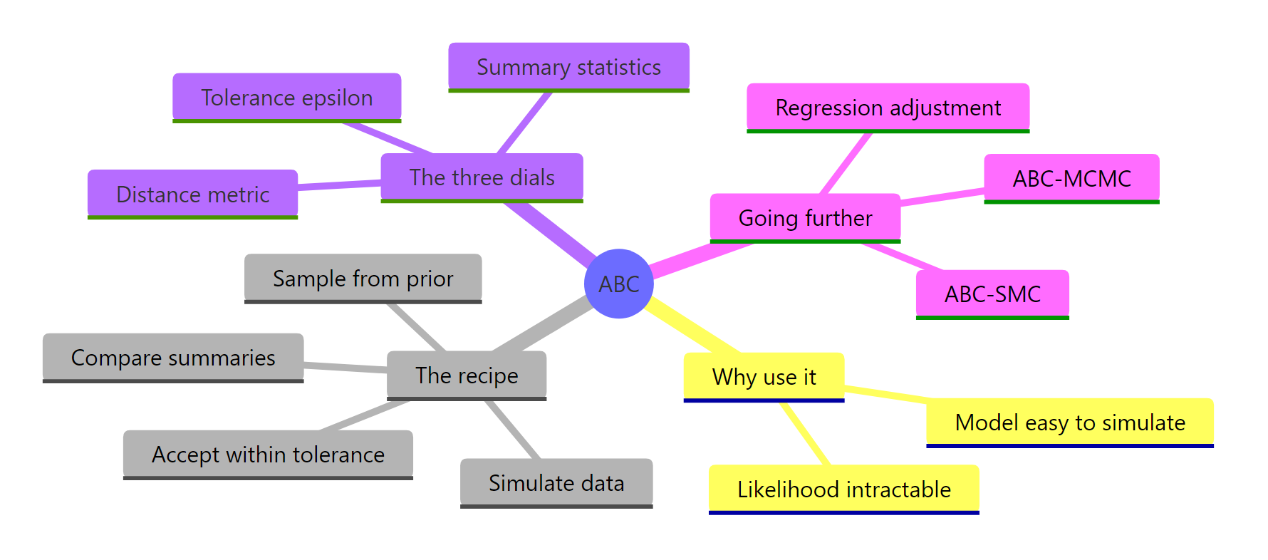
Figure 2: The moving parts of ABC at a glance.
| Idea | What to remember |
|---|---|
| Core trick | Replace evaluating the likelihood with simulating data and keeping the parameters that reproduce it |
| When to use it | The model is easy to simulate but its likelihood is intractable or unknown |
| The four steps | Draw from the prior, simulate, reduce to summary statistics, accept within tolerance |
| Summary statistics | Raw data never matches, so compare compact summaries; choose ones that carry information about the parameters |
| Tolerance epsilon | Smaller tolerance means a more accurate but more expensive posterior; as it goes to zero, ABC becomes exact |
| Verification | On the coin, ABC reproduced the exact Beta posterior to two decimals, which is why we trust it on likelihood-free models |
| Making it efficient | ABC-MCMC and ABC-SMC waste fewer simulations; regression adjustment sharpens a cheap, loose run for free |
| In practice | The abc and EasyABC packages implement all of this; you now know the machinery inside them |
References
- Marin, J.-M., Pudlo, P., Robert, C. P., Ryder, R. J. - Approximate Bayesian computational methods. Statistics and Computing 22, 1167-1180 (2012). A broad survey of ABC algorithms and their theory, one step up from this post. Link
- Beaumont, M. A., Zhang, W., Balding, D. J. - Approximate Bayesian Computation in Population Genetics. Genetics 162, 2025-2035 (2002). The paper that introduced the regression-adjustment step used in the efficiency section. Link
- Sisson, S. A., Fan, Y., Beaumont, M. A. (eds.) - Handbook of Approximate Bayesian Computation. Chapman and Hall/CRC (2018). The reference handbook, covering the rejection, MCMC, and SMC variants in depth. Link
- Sunnaker, M. et al. - Approximate Bayesian Computation. PLoS Computational Biology 9(1): e1002803 (2013). An open-access primer with worked biological examples, good for a gentle second pass. Link
- Csillery, K., Francois, O., Blum, M. G. B. - abc: an R package for Approximate Bayesian Computation. Methods in Ecology and Evolution 3, 475-479 (2012). Documents the abc package that automates the rejection and regression steps you built here by hand. Link
- Jabot, F., Faure, T., Dumoulin, N. - EasyABC: an R package to perform efficient approximate Bayesian computation. Documents EasyABC, which implements the ABC-MCMC and ABC-SMC schemes named in the efficiency section. Link
- Pritchard, J. K., Seielstad, M. T., Perez-Lezaun, A., Feldman, M. W. - Population growth of human Y chromosomes: a study of Y chromosome microsatellites. Molecular Biology and Evolution 16, 1791-1798 (1999). One of the earliest applications of the ABC rejection idea, in population genetics. Link
Continue Learning
- MCMC in R: Metropolis-Hastings from Scratch - the likelihood-based sampler ABC replaces when the likelihood is out of reach.
- Variational Bayes in R: Fast Approximate Inference - another way to approximate a posterior, this time by optimization instead of simulation.
- Bayesian Statistics in R - the priors, likelihoods, and posteriors that ABC quietly rests on.