Credible vs Confidence Intervals in R
A confidence interval and a credible interval can print almost the same two numbers, yet they answer different questions. A 95% confidence interval is a statement about a procedure repeated many times: cast the net this way and 95% of the nets you cast will catch the true value. A 95% credible interval is the statement people usually want: given this data, there is a 95% probability the true value sits inside the range. This post computes both on the same data using plain base R, shows why they usually agree, and shows the cases where they clearly split apart.
What is the difference between a credible interval and a confidence interval?
The difference is not in the arithmetic. It is in what you are allowed to say once you have the two numbers. To make that concrete, we will carry one small example through the whole post: a landing page shows a signup button to 40 visitors, and 12 of them convert. We want a range for the true conversion rate.
Let us compute both 95% intervals right away and put them side by side. One is the frequentist confidence interval from binom.test(). The other is the Bayesian credible interval, which we get by starting from a flat "no opinion" prior and reading the middle 95% of the resulting posterior. Do not worry about how the Bayesian one works yet; we build it up properly in a few sections. For now, just watch the numbers.
Here is what that code did. It stored the counts in x and n, asked binom.test() for the exact 95% confidence interval, then built the credible interval with qbeta(), which reads quantiles straight off a Beta distribution. The two rows are the two intervals.
Now read them. The confidence interval runs from 0.166 to 0.465. The credible interval runs from 0.181 to 0.455. They are close enough that on a chart you would struggle to tell them apart. So if the numbers are almost the same, why does anyone argue about which to use? Because the sentence you are entitled to say about each one is completely different.
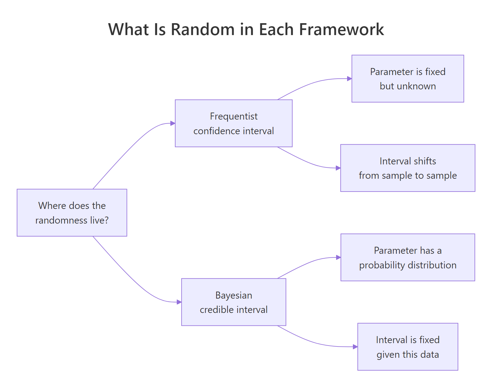
Figure 1: In the frequentist view the parameter is fixed and the interval is random; in the Bayesian view the parameter is random and the interval is fixed.
The picture captures the whole disagreement. A frequentist treats the true conversion rate as one fixed number that we simply do not know. What is random is the interval: run the test again with 40 fresh visitors and you get slightly different counts, so you get a slightly different interval. A Bayesian flips it. The data you collected is fixed, so the interval is fixed, and the unknown rate is described by a probability distribution.
Try it: The two intervals above are stored in ci and cri. Measure how wide each one is (upper bound minus lower bound) and round to 3 decimals.
Click to reveal solution
Explanation: Both intervals span roughly three-tenths of the 0-to-1 scale, which tells you 40 visitors is not much data. The credible interval is a hair narrower here, but with this much data the difference is cosmetic.
What does a 95% confidence interval actually mean?
The confidence interval has the interpretation that trips up almost everyone, so it is worth slowing down. The claim is about repetition. Imagine you could rerun the exact same test thousands of times, each time with 40 new visitors drawn from the same true rate. Each run produces its own confidence interval. The "95%" promises that about 95 out of every 100 of those intervals would contain the true rate.
That is a claim we can check by simulation, and checking it makes the idea stick. We will fix a true rate of 0.30, generate 2000 pretend experiments, build a confidence interval for each, and count how often the interval actually captured 0.30. We use set.seed() so the random draws are reproducible.
Walk through the loop. Each pass simulates one experiment with rbinom(), which draws a number of successes out of n visitors at the true rate. It builds that experiment's confidence interval, then records TRUE if 0.30 fell inside. Averaging those TRUE/FALSE results gives the fraction of intervals that caught the truth.
The answer is 0.9655, about 96.6% of the intervals. That is the confidence guarantee in action. It landed a little above 95% because binom.test() uses the exact interval, which is built to never dip below 95% coverage and so usually sits slightly above. The headline is the mechanism: the 95% lives in the long-run success rate of the procedure, not in any single interval you compute.
Try it: Repeat the simulation with a true rate of 0.5 instead of 0.30. Keep n at 40 and use 2000 repetitions. Does the coverage stay in the same ballpark?
Click to reveal solution
Explanation: Coverage is 0.962, again just above 95%. The guarantee holds across different true rates, which is exactly what "works 95% of the time in the long run" is supposed to mean.
What does a 95% credible interval actually mean?
The credible interval gives you the sentence the confidence interval refuses to give: there is a 95% probability the true rate is inside this range. It can say that because it treats the unknown rate as a quantity with a probability distribution, updated by your data.
That distribution is called the posterior, and it comes from combining two things. The first is the prior, your belief about the rate before seeing data. The second is the likelihood, what the 12-out-of-40 result says on its own. For a rate between 0 and 1 with count data, a flat Beta(1, 1) prior (which treats every rate as equally plausible) plus x successes and n - x failures gives a posterior that is again a Beta distribution: Beta(1 + x, 1 + n - x). The credible interval is just the middle 95% of that curve.
Read the four numbers. The posterior is centered at 0.310, close to the raw rate of 12/40. Its middle 95% runs from 0.181 to 0.455, which is the credible interval. And because we have a full distribution, we can answer questions a confidence interval cannot: the posterior probability that the true rate is above 0.25 is 0.794, or about 79%. That last line is a direct probability statement about the parameter, and it is completely legitimate in the Bayesian world.
A picture makes the interval concrete. The shaded band below is the region that holds 95% of the posterior's area.
The dashed lines mark the 2.5% and 97.5% cutoffs. Everything between them is the credible interval, and the shaded area under the curve there is exactly 0.95.
If you like the formula behind the picture, here it is. The intuition is that the posterior is the prior reweighted by how well each rate explains the data.
$$p(\theta \mid \text{data}) \; \propto \; p(\text{data} \mid \theta)\; p(\theta)$$
Where:
- $p(\theta \mid \text{data})$ = the posterior, your updated belief about the rate $\theta$ after seeing the data
- $p(\text{data} \mid \theta)$ = the likelihood, how probable the observed 12-of-40 is at each rate $\theta$
- $p(\theta)$ = the prior, your belief about $\theta$ before the data
- the $\propto$ ("proportional to") sign hides a constant that just rescales the curve so its area is 1
If formulas are not your thing, skip the equation. The shaded plot already told the whole story: prior in, data in, posterior out, and the credible interval is the middle 95% of it.
Try it: Using the same posterior, compute the probability that the true rate is below 0.20. The function pbeta(q, a_post, b_post) gives the area to the left of q.
Click to reveal solution
Explanation: There is only a 5.2% posterior probability the true rate is below 0.20. That fits the interval you already saw: 0.181 is the lower 2.5% cutoff, so a bit more than 2.5% of the curve sits below 0.20.
How do you compute each interval in R?
Now that you know what each interval means, here are the practical recipes side by side. Confidence intervals for a proportion come in a few flavors, and it helps to see them together. We will compute the exact interval from binom.test(), the Wilson interval from prop.test(), and the plain Wald interval by hand.
The three rows agree to within a couple of hundredths here because 40 is a comfortable sample size. The Wald row came from a formula you can write on a napkin: take the observed rate and step out by a z-score's worth of standard error on each side.
$$\hat{p} \; \pm \; z_{0.975}\sqrt{\frac{\hat{p}\,(1 - \hat{p})}{n}}$$
Where:
- $\hat{p}$ = the observed success rate,
x / n - $z_{0.975} \approx 1.96$ = the standard-normal cutoff that leaves 2.5% in each tail
- $n$ = the number of trials
For the credible interval, there are also two natural routes, and they should give the same answer. The first reads quantiles straight off the Beta posterior with qbeta(). The second draws a large sample from the posterior with rbeta() and takes empirical quantiles. Simulation is the route you fall back on when a posterior has no tidy formula.
They match to three decimals, which confirms the simulation route works whenever you cannot solve the posterior by hand. So far every credible interval has been "equal-tailed," meaning we chopped off 2.5% from each side. There is a second style called the highest density interval, or HDI, which instead finds the shortest interval that still holds 95% of the posterior. For a skewed posterior the HDI can be noticeably tighter. Here is a small helper that finds it from the samples.
The HDI slides slightly left, from [0.181, 0.455] to [0.176, 0.449], because this posterior leans a touch to the right and the shortest window trims a little off the long tail. For a nearly symmetric posterior like this one the two barely differ; the gap grows when the posterior is strongly skewed.
Try it: Compute an 80% equal-tailed credible interval instead of a 95% one. An 80% interval leaves 10% in each tail, so use the 10% and 90% quantiles with qbeta().
Click to reveal solution
Explanation: The 80% interval, [0.221, 0.402], is narrower than the 95% one because it is willing to be wrong more often. Lower confidence always buys you a shorter interval.
When do credible and confidence intervals give different answers?
So far the two intervals have been near twins. That is the common case: with a fair amount of data and a flat prior, they nearly coincide. The disagreements show up in two situations, and both are worth recognizing.
The first is a small sample near a boundary. Suppose a feature was shown to just 5 users and none of them clicked: 0 successes out of 5. Watch what each method does.
The Wald interval collapses to the single point [0, 0], claiming with 95% confidence that the true rate is exactly zero. That is nonsense: five clicks-free visitors hardly prove the button never works. The exact confidence interval behaves sensibly, stretching up to 0.522. The credible interval also behaves sensibly, [0.004, 0.459], and it even nudges the lower bound off zero because a flat prior still assigns some probability to small positive rates. Near a boundary, the method you pick matters a lot.
The second source of disagreement is a strong prior. A confidence interval cannot use prior information even when you have some; a credible interval can, and it will move the answer. Suppose past launches make you skeptical, so you bring a Beta(2, 18) prior with mean 0.1 (worth about 20 pretend trials). Compare it against the confidence interval and the flat-prior credible interval on our original 12-of-40 data.
The skeptic's interval, [0.136, 0.347], has slid clearly below the other two. Its prior belief that the rate is around 0.1 pulled the whole range down. The confidence interval, by design, ignored that outside knowledge entirely. Whether pulling the answer down is right or wrong depends on whether the skeptical prior was defensible, which is exactly the judgment call a confidence interval never asks you to make.
Try it: Flip the skeptic into an optimist. Use a Beta(18, 2) prior (mean 0.9), add the 12 successes and 28 failures, and read the 95% credible interval.
Click to reveal solution
Explanation: The optimistic prior is worth 20 pretend trials pulling toward 0.9, so it drags the interval up to [0.375, 0.625], centered near 0.5 rather than the data's 0.3. A strong prior has a large effect when the data are modest, which is precisely why prior choice deserves scrutiny.
Which interval should you use?
The honest answer is that for most well-powered analyses it barely matters, because the two intervals nearly coincide and point to the same decision. When they do differ, the choice comes down to two questions: do you have prior information worth using, and what sentence do you need to say?
Reach for a confidence interval when you want a purely objective summary that uses only the data in front of you, or when your audience expects the frequentist standard. Reach for a credible interval when you have a defensible prior worth including, or when you need to state a genuine probability about the parameter, such as "there is a 90% chance the rate beats our target."
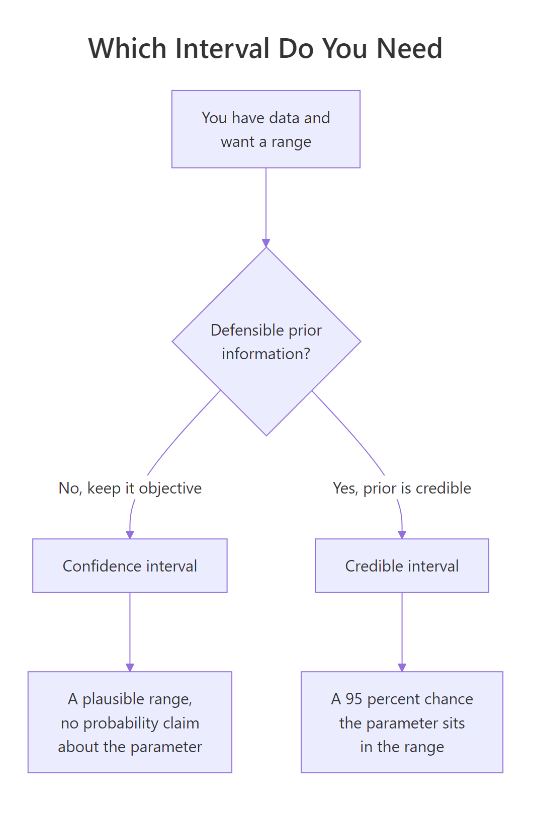
Figure 2: A quick rule for choosing between a confidence interval and a credible interval.
There is a practical shortcut that sidesteps the philosophy entirely: if both intervals lead to the same decision, you do not need to pick a winner. Say your launch target is a 25% conversion rate and you will ship only if you are confident the true rate clears it. Check whether each interval sits entirely above 0.25.
Both come back FALSE: neither interval sits fully above 0.25, because both lower bounds (0.166 and 0.181) fall short of the target. The two frameworks agree that 12 of 40 is not yet enough evidence to declare the target beaten. When both endpoints tell the same story, the decision is settled and the frequentist-versus-Bayesian debate is moot.
Try it: Rerun the same-decision check against a lower target of 0.15. Do the intervals clear that bar?
Click to reveal solution
Explanation: Against the easier 0.15 target both intervals return TRUE, since their lower bounds (0.166 and 0.181) clear 0.15. Again the two agree, so you can act without ever settling the philosophical question.
Putting it all together: a complete comparison
Let us run the full workflow once on a fresh dataset so you can see every piece in one place. A button was shown to 50 users and 30 clicked. We will compute both 95% intervals, then lay them out in a table and draw them on one axis.
The two centers (0.600 and 0.596) are almost identical, and the two ranges overlap heavily. With 50 data points and a flat prior, the frameworks have essentially converged, which is the typical outcome once you leave the small-sample corner. Drawing them makes the overlap obvious.
The two bars sit almost on top of each other. That single image is the practical takeaway of the whole post: most of the time the intervals agree on the numbers, and the real difference is the sentence you are allowed to attach to them.
Practice Exercises
These combine the ideas above. Try each before opening the solution. The exercises use their own my_ variables so they will not disturb the objects from the tutorial.
Exercise 1: Compare both intervals on a tiny sample
A quick poll finds that 7 of 10 people preferred version B. Compute both 95% intervals for the true preference rate, then compare their widths. Which interval is wider, and why does that make sense with only 10 responses?
Click to reveal solution
Explanation: With only 10 responses both intervals are very wide, spanning half the scale or more. The exact confidence interval (width 0.586) is the wider of the two because it is built to guarantee at least 95% coverage, which makes it deliberately cautious. The flat-prior credible interval (width 0.500) is a bit tighter.
Exercise 2: Write a reusable interval function
Write a function both_intervals(x, n, level) that returns the exact confidence interval and the flat-prior credible interval as a two-row matrix. Then test it on a rare event: 3 successes in 100 trials at the default 95% level.
Click to reveal solution
Explanation: The function turns the two recipes into one call. On 3-in-100 both intervals land near [0.01, 0.085], reassuringly close because the flat prior adds almost nothing against 100 trials. The conf.level = level and qbeta(c(a, 1 - a), ...) pieces let the same function serve any confidence level.
Exercise 3: Show how a prior moves the answer
Priors matter most when data is thin. For the same 3 successes in 100 trials, compute the 95% credible interval under a flat Beta(1, 1) prior and under an informative Beta(10, 10) prior that believes the rate is near 0.5. How far does the informative prior pull the interval?
Click to reveal solution
Explanation: The Beta(10, 10) prior is worth 20 pretend trials pulling toward 0.5, so even against 100 real trials it drags the interval up from about [0.011, 0.084] to [0.059, 0.170]. With a defensible prior that pull is a feature; with an indefensible one it is a bug, which is why prior choice deserves scrutiny whenever data is scarce.
Frequently Asked Questions
Is a credible interval the same as a Bayesian confidence interval?
People sometimes call it a "Bayesian confidence interval," but the proper name is credible interval, and the distinction is not just vocabulary. A credible interval comes from a posterior distribution and supports a direct probability statement about the parameter. A confidence interval comes from the sampling behavior of an estimator and does not. Using the two names interchangeably invites exactly the misinterpretation this post is trying to prevent.
Does a 95% confidence interval mean a 95% probability the parameter is inside?
No, and this is the single most common mistake. For a specific computed confidence interval, the true parameter is either inside or outside; there is no probability left to assign. The 95% refers to the long-run success rate of the procedure across many repeated samples, as the coverage simulation showed. The only interval that carries a genuine 95% probability for the parameter is the credible interval.
What is the difference between an equal-tailed and a highest density interval?
An equal-tailed interval leaves the same probability in each tail, for a 95% interval that is 2.5% below and 2.5% above. A highest density interval is the shortest interval that still contains 95% of the posterior, and every point inside it has higher density than any point outside. For a symmetric posterior the two coincide; for a skewed one the highest density interval is tighter and can sit noticeably off-center.
Do I always need a prior to build a credible interval?
Yes, a credible interval is defined by the posterior, and the posterior needs a prior. The flat Beta(1, 1) prior used throughout this post is a common "let the data speak" default, and with a reasonable sample it produces intervals nearly identical to the confidence interval. When data is scarce the prior matters more, so it is worth choosing deliberately and checking how sensitive your answer is to it.
Which one should I report for an A/B test?
Either works, and with a healthy sample size they will agree. Pick the credible interval when you want to say something like "there is a 92% probability B beats A," which stakeholders find easy to act on. Pick the confidence interval when your organization or reviewers expect the frequentist standard. If the two disagree, that is a cue your sample is small or a prior is influential, and either way you should gather more data before deciding.
Summary
The table below distills the whole comparison into the points worth remembering.
| Question | Confidence interval | Credible interval |
|---|---|---|
| What is random? | The interval (parameter is fixed) | The parameter (interval is fixed) |
| Interpretation of 95% | 95% of such intervals catch the truth | 95% probability the truth is in this range |
| Needs a prior? | No | Yes |
| Direct probability claim about the parameter? | Not allowed | Allowed |
| R starting point (proportion) | binom.test(), prop.test() |
qbeta() on a Beta posterior |
| Typical result with good data | Nearly identical | Nearly identical |
| When they diverge | Small samples, boundaries, strong priors | Small samples, boundaries, strong priors |
The practical bottom line: compute both when it is cheap, and if they lead to the same decision you are done. When they disagree, the gap is pointing at a small sample or an influential prior, and that is information worth having before you act.
References
- Wikipedia. Credible interval. Link
- Wikipedia. Confidence interval. Link
- R Core Team. binom.test: Exact Binomial Test (stats package reference). Link
- R Core Team. prop.test: Test of Equal or Given Proportions (stats package reference). Link
- bayestestR. Credible Intervals (CI) vignette (easystats, equal-tailed and highest density intervals in R). Link
- Morey, R. D., Hoekstra, R., Rouder, J. N., Lee, M. D., Wagenmakers, E.-J. The Fallacy of Placing Confidence in Confidence Intervals. Psychonomic Bulletin & Review (2016). Link
- VanderPlas, J. Frequentism and Bayesianism III: Confidence, Credibility, and why Frequentism and Science do not Mix. Link
Continue Learning
- Confidence Intervals in R - a deeper tour of frequentist intervals for means and proportions.
- Bayesian Statistics in R - how priors, likelihoods, and posteriors fit together across models.
- Posterior Predictive Checks in R - once you trust your posterior, check whether the model actually fits the data.