ACF and PACF in R: How to Read the Plots for ARIMA Orders
The ACF (autocorrelation function) measures how strongly each value in a time series correlates with its own past at every lag. The PACF (partial autocorrelation function) measures that same correlation after stripping out the shorter lags in between. Read the two plots together and their shape hands you the p and q orders for an ARIMA model.
That last sentence is the whole promise of this guide, and by the end you will be able to keep it. We will use base R plus the forecast package, and every plot you meet here comes from a series where we already know the true answer, so you can check the reading against reality before you trust it on your own data.
What do the ACF and PACF actually measure?
Before you can read a single plot, you need to know what those bars stand for. Autocorrelation is nothing exotic: it is ordinary correlation applied to a series and a shifted copy of itself. We will compute one by hand on eight numbers, then let R reproduce it, so the plot later is never a black box.
Here is the idea in code. We take a short series, line it up against a copy of itself shifted back by one step, and measure how tightly the two move together.
The value 0.456 is the lag-1 autocorrelation. It is positive and fairly large, which says that a high value tends to be followed by another high value. That is the entire concept: autocorrelation at lag k is how much the series at time t looks like the series k steps earlier.
You will never compute this by hand again, because R does it for every lag at once. The acf() function returns the whole set, from lag 0 upward.
Read the lag-1 entry: 0.456, exactly the number we built by hand. Lag 0 is always 1.000 (a series is perfectly correlated with itself), so it carries no information and the plots you meet later hide it. The autocorrelation then fades to 0.232 at lag 2 and drifts negative by lag 4.
If you like the formal version, the autocorrelation at lag $k$ is
$$r_k = \frac{\sum_{t=k+1}^{n} (y_t - \bar{y})(y_{t-k} - \bar{y})}{\sum_{t=1}^{n} (y_t - \bar{y})^2}$$
Where $y_t$ is the series, $\bar{y}$ is its mean, and $k$ is the lag. That is the exact recipe our by-hand code followed. If formulas are not your thing, skip it: the code above is all you need.
The PACF answers a subtler question. The lag-2 autocorrelation is partly secondhand: y_t relates to y_{t-1}, and y_{t-1} relates to y_{t-2}, so some of the lag-2 link is just the lag-1 link passed down the chain. Think of the height correlation between grandparents and grandchildren, much of which runs through the parents. The partial autocorrelation at lag 2 strips out that middle-man effect and reports only the direct grandparent-to-grandchild link. That distinction is exactly what separates AR order from MA order later.
Try it: Measure the direct-plus-indirect link at lag 2 on the same eight numbers. Pair ex_x[3:8] with ex_x[1:6] (both centred by their mean) and confirm you get the lag-2 value from the acf() table above.
Click to reveal solution
Explanation: Shifting by two steps pairs the 3rd-through-8th values with the 1st-through-6th. The result, 0.232, matches the lag-2 entry from acf(), which is the reassuring point: the function is just doing this arithmetic for you.
How do you plot the ACF and PACF in R, and what are the blue dashed lines?
Numbers in a table are hard to scan, so in practice you read pictures. R gives you two base functions, acf() and pacf(), and the forecast package adds prettier, gg-style versions: Acf(), Pacf(), and the all-in-one ggtsdisplay(), which stacks the series, its ACF, and its PACF in a single frame.
Let's generate a series whose true order we know so we have a benchmark. We simulate 200 points from an autoregressive process where each value leans 0.7 on the one before it, then display all three panels at once.
The top panel is the wandering series. The bottom-left panel is the ACF, and the bottom-right is the PACF. Each bar is a correlation at that lag. The pair of blue dashed lines is the part everyone squints at, so let's pin down exactly what they are.
The dashed lines mark the range where a bar is "basically zero", meaning indistinguishable from the wiggles you would see in pure noise. They sit at
$$\pm \frac{1.96}{\sqrt{n}}$$
Where $n$ is the number of observations. A bar poking outside the band is a genuine signal; a bar inside is noise you should ignore. For our 200-point series the band is:
So any bar taller than about 0.139 (or lower than -0.139) counts. That single number turns plot-reading from guesswork into a rule: compare each bar against the band and ask, in or out?
Acf() and Pacf() from the forecast package start their tables at lag 1 because the lag-0 bar is always 1 and only squashes the interesting bars. Base acf() includes lag 0. Nothing else differs, so use whichever reads more clearly.Try it: The built-in lh series (luteinizing hormone, 48 samples) is shorter than our simulated one. Work out where its dashed band would sit.
Click to reveal solution
Explanation: With only 48 points the band widens to 0.283, more than double the band for our 200-point series. Fewer observations means more uncertainty, so bars must be taller to count. Always read a plot against its own band, never a remembered number.
What do "cutoff" and "tail off" mean on these plots?
Two words carry the entire method, so let's make them concrete. A plot cuts off when its bars drop abruptly inside the band after some lag and stay there. A plot tails off when its bars shrink gradually, lag after lag, sometimes decaying smoothly and sometimes oscillating as they fade.
Our ar1 series shows one of each. Look at its ACF as numbers first.
The bars shrink smoothly: 0.666, then 0.407, then 0.177, each roughly 0.6 times the last. That gradual fade is a textbook tail-off. Nothing cuts; it just decays toward the band.
Now the PACF of the very same series.
Completely different shape. One tall bar at lag 1 (0.666, well outside the 0.139 band), then everything collapses inside the band and stays there. That abrupt drop after lag 1 is a cutoff. One plot tails off, the other cuts off, from identical data. That contrast is the fingerprint you will read for the rest of this guide.
Here is the map you are about to fill in. Over the next three sections we work through each of these four fingerprints and the model it points to.
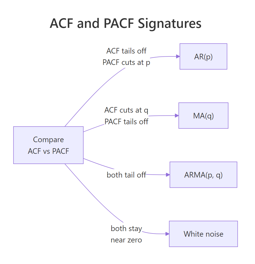
Figure 1: The four ACF/PACF fingerprints and the model each one points to.
Try it: Print just the first five partial autocorrelations of ar1 and name the lag where the plot cuts off.
Click to reveal solution
Explanation: Only lag 1 (0.666) clears the band. Lags 2 through 5 all sit inside it, so the PACF cuts off after lag 1. In the next section you will see that a PACF cutting off at lag 1 is the signature of an AR(1) process, which is exactly how we built this series.
How do you read the AR order (p) from the PACF?
An autoregressive process of order p, written AR(p), predicts each value from its own previous p values. Its fingerprint is fixed and reliable: the ACF tails off, and the PACF cuts off at lag p. So to find p, you look at the PACF and count how many bars stand outside the band before it collapses.
Let's prove it on a series we build to be AR(2), where each value depends on the two before it.
The ACF panel tails off gradually, as it did for AR(1). The PACF panel is where you read the order. Let's see it as numbers.
With 300 points the band is about 0.113. Lags 1 (0.767) and 2 (0.299) clear it comfortably; lag 3 (-0.103) falls just inside; everything after is noise. The PACF cuts off after lag 2, so you read p = 2, which matches the process we simulated. The rule is simply: the last PACF bar outside the band is your p.
Try it: Simulate a series that depends on its previous three values (an AR(3)) and read p from the PACF.
Click to reveal solution
Explanation: With 400 points the band is about 0.098. Lags 1, 2, and 3 (0.554, 0.303, 0.250) all clear it, then lag 4 drops inside, so the cutoff is at lag 3 and p = 3. Notice lag 7 (0.105) pokes a hair outside the band too. That is a chance spike, not a real order-7 term: with many lags, roughly 1 in 20 will cross the band by luck, so ignore isolated bars far from the others.
How do you read the MA order (q) from the ACF?
A moving-average process of order q, written MA(q), builds each value from the last q random shocks rather than the last q values. Its fingerprint is the mirror image of the AR case: the ACF cuts off at lag q, and the PACF tails off. So for q you read the ACF, not the PACF.
Let's watch it happen on a series built to be MA(1).
This time the roles swap: the PACF panel decays gradually while the ACF panel has one spike and then nothing. Read the ACF as numbers to confirm.
Lag 1 (0.459) clears the 0.113 band; lag 2 (-0.064) is already inside; the rest is noise. The ACF cuts off after lag 1, so q = 1, exactly the process we simulated.
Try it: Simulate an MA(2), where each value carries two shocks, and read q from its ACF.
Click to reveal solution
Explanation: Lags 1 (0.601) and 2 (0.270) sit outside the 0.098 band, then lag 3 (0.019) drops inside. The ACF cuts off after lag 2, so q = 2, the order we built.
What if both plots tail off? Reading a mixed ARMA
Real data is rarely as tidy as a pure AR or pure MA. When a process has both autoregressive and moving-average parts, an ARMA(p, q), neither plot gives you a clean cutoff. Both the ACF and the PACF tail off. That is itself a signature: gradual decay in both plots tells you that you need both kinds of term.
Let's simulate an ARMA(1,1) and look.
Neither panel snaps to zero after a lag or two; both fade out. When you see this, stop trying to count bars, because the exact p and q are not visible in the plots. Instead you fit a few small candidate models and let an information criterion pick the best trade-off between fit and simplicity. The auto.arima() function does exactly that search.
Interesting result worth pausing on. We simulated an ARMA(1,1), but the search picked ARIMA(2,0,0), a pure AR(2). That is not a bug. An ARMA(1,1) can be closely mimicked by an AR(2), and here the simpler AR(2) scored a lower AICc, so it won. This is the honest reality of mixed processes: several orders fit almost equally well, which is precisely why the plots alone cannot settle it and why you confirm your choice later with residual checks.
Try it: Compare the AICc of an AR(2) and an ARMA(1,1) fit to arma11 and see which the criterion prefers.
Click to reveal solution
Explanation: The AR(2) scores 1108.59 against the ARMA(1,1) at 1112.66. Lower is better, so AICc prefers the AR(2), which is why auto.arima() chose it. When the plots are ambiguous, this numeric comparison is your tie-breaker.
How does the ACF tell you when to difference (the d in ARIMA)?
Everything so far assumed the series is stationary, meaning its mean and variance do not drift over time. If a series trends or wanders, the ACF and PACF rules break down, and the ACF itself is what warns you. A non-stationary series shows an ACF that stays high and decays very slowly, almost in a straight line, across many lags.
The d in ARIMA is the number of times you difference the series (subtract each value from the next) to remove that drift. Let's build a random walk, the classic non-stationary series, and look at its ACF.
The series clearly wanders with no fixed level. Its ACF tells the same story in numbers.
That is the tell-tale sign: 0.920, 0.850, 0.792, a long, slow, nearly linear slide. The series does not tend back toward a fixed level, so distant values stay strongly correlated. The fix is to difference once and re-check.
One difference and the slow decay is gone: every bar from lag 1 on sits inside the band. The differenced series is white noise, which for a random walk is exactly right, and it tells you d = 1. The workflow is always this: if the ACF decays slowly, difference the series, then read the ACF and PACF of the differenced version for p and q. (If you want the formal stationarity tests that back up this visual check, see Test for Stationarity in R.)
Try it: Difference the random walk one time too many and watch the over-differencing signature appear at lag 1.
Click to reveal solution
Explanation: One difference already made the random walk stationary. The second difference over-does it, and the lag-1 autocorrelation drops to -0.507, the classic strong-negative signal of an over-differenced series. Lesson: difference the minimum number of times that removes the slow decay, and no more.
How do you handle seasonal spikes in the ACF and PACF?
Many real series repeat on a calendar: monthly sales peak every December, temperatures cycle every 12 months. Seasonality leaves an unmistakable mark: the ACF shows spikes at multiples of the seasonal period, for example at lags 12, 24, and 36 for monthly data.
The built-in AirPassengers series counts monthly airline passengers and has both a rising trend and a yearly cycle. We difference once to strip the trend so the seasonal pattern stands out cleanly, then plot the ACF out to 36 lags.
The bars rise sharply at lags 12, 24, and 36, one big spike per year. Read those same lags as numbers to see the size of the seasonal correlation.
Lag 12 stands at 0.829, far above its neighbours. That single dominant spike at the seasonal period is your cue to add a seasonal term, which in a full model means moving from ARIMA to seasonal ARIMA (SARIMA). The same cutoff-versus-tail-off reading then applies again, but at the seasonal lags 12, 24, 36 instead of 1, 2, 3.
Try it: Apply a seasonal difference (lag 12) on top of the regular difference and check whether the giant lag-12 spike has collapsed.
Click to reveal solution
Explanation: After the seasonal difference the lag-12 autocorrelation falls from 0.829 all the way to -0.134, inside the band. The yearly spike is gone, which tells you a seasonal difference (a seasonal d of 1) was the right move. What remains at the low lags is the ordinary, non-seasonal structure you read as before.
Complete example: choose and confirm an ARIMA order
You now have every piece. Let's run the whole workflow end to end on a real dataset you have not seen, following the loop below from raw series to a confirmed model.

Figure 2: The order-identification loop from raw series to a confirmed model.
The LakeHuron series records the water level of Lake Huron in feet, once a year from 1875 to 1972. First, look at it.
The level drifts around a stable range without a strong trend, so it looks stationary enough to read directly, meaning we can try d = 0. Next, the two diagnostic plots.
The ACF tails off gradually and the PACF cuts off early. That is the AR signature, so we read p from the PACF.
With 98 observations the band is about 0.198. Lag 1 (0.832) and lag 2 (-0.267) clear it; lag 3 (0.131) sits inside. The PACF cuts off after lag 2, so our candidate is ARIMA(2, 0, 0). The three numbers in that order are always (p, d, q): here p = 2 (the AR order we just read from the PACF), d = 0 (no differencing, since the series is already stationary), and q = 0 (no MA term). The Arima() function takes exactly that vector as its order argument. Now fit it.
Both AR coefficients are several standard errors from zero, which is a good sign the order is real. But a model that fits is not yet a model you trust. The final check is the residuals: if the model captured all the structure, what is left over should be white noise, with an ACF that stays inside the band. The checkresiduals() function plots that residual ACF and runs the Ljung-Box test, which asks a single question, are the residual autocorrelations jointly indistinguishable from zero?
The Ljung-Box p-value is 0.6533, comfortably above 0.05. A high p-value here is the good outcome: it means we cannot reject the idea that the residuals are white noise, so no autocorrelation is left unexplained. Our ARIMA(2, 0, 0), read straight off the PACF, is confirmed.
p or q and refit.Practice Exercises
These combine several steps. Try each before opening the solution, and note the distinct variable names so your work does not clash with the tutorial's series.
Exercise 1: Identify a moving-average order
Simulate a series with two moving-average terms and read its order. Decide first which plot carries the answer, then read q from it.
Click to reveal solution
Explanation: This is a moving-average process, so the order lives in the ACF. Lags 1 (0.342) and 2 (-0.127) clear the 0.098 band, then lag 3 (0.048) drops inside. The ACF cuts off after lag 2, so q = 2, which matches the two MA terms we simulated.
Exercise 2: Run the full workflow on real data
The built-in lh series has 48 samples of luteinizing hormone. Run the complete loop: inspect the ACF and PACF, pick an order, fit it, and confirm with the Ljung-Box test.
Click to reveal solution
Explanation: The band for 48 points is 0.283. Only lag 1 of the PACF (0.576) clears it, so the PACF cuts off after lag 1 and p = 1. The series has no slow-decaying ACF, so d = 0. Fitting ARIMA(1, 0, 0) gives a Ljung-Box p-value of 0.405, well above 0.05, so the residuals are white noise and the order is confirmed.
Exercise 3: Tell AR(1) from MA(1)
Here are two mystery series simulated for you. One is AR(1), the other is MA(1). Use the cutoff-versus-tail-off fingerprint to decide which is which.
Click to reveal solution
Explanation: Series A has an ACF that tails off smoothly (0.846, 0.700, 0.563) while its PACF cuts off after lag 1. That is the AR signature, so A is AR(1). Series B is the mirror image: its ACF cuts off after lag 1 (0.389, then inside the band) while its PACF tails off with an oscillating decay. That is the MA signature, so B is MA(1). Same fingerprint logic, opposite plots.
Summary
Reading the ACF and PACF comes down to spotting which plot cuts off and which tails off, then matching that pair to a model. The table collects every signature in one place.
| ACF pattern | PACF pattern | Model | Where you read the order |
|---|---|---|---|
| Tails off | Cuts off after lag p | AR(p) | PACF |
| Cuts off after lag q | Tails off | MA(q) | ACF |
| Tails off | Tails off | ARMA(p, q) | Fit + AICc |
| Decays very slowly | Stays high | Non-stationary | Difference, then re-read |
| Spike at lag 12, 24 | Spike at lag 12, 24 | Seasonal (SARIMA) | Seasonal lags |
A few rules make the reading reliable: compare every bar against that series' own 1.96/sqrt(n) band; the last bar outside the band on the cutting-off plot is your order; slow ACF decay means difference before you read; and whatever order you pick, confirm it by checking the model's residuals are white noise. The mind map ties the whole method together.
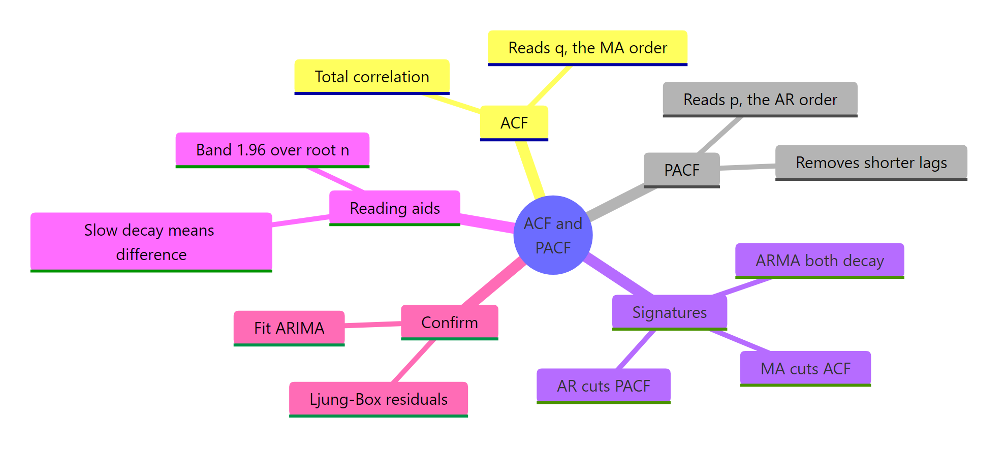
Figure 3: How the ACF, PACF, signatures, and confirmation steps fit together.
Frequently Asked Questions
Do I read the AR order from the ACF or the PACF? From the PACF. The PACF cuts off at the AR order p, while the ACF tails off. For the MA order q it is the other way around: read the ACF, which cuts off at q, while the PACF tails off. A handy mnemonic is "PACF for p, ACF for q".
What do the blue dashed lines on an ACF or PACF plot mean? They mark the significance band at plus or minus 1.96/sqrt(n), where n is the number of observations. A bar that stays inside the band is statistically indistinguishable from zero, so treat it as noise. Only bars that poke outside the band count as real correlation.
What does it mean when both the ACF and the PACF tail off? That is the signature of a mixed ARMA process, which needs both AR and MA terms. The plots cannot hand you exact orders in this case, so fit a few small candidates (start near ARIMA(1,0,1)) and pick the one with the lowest AICc, then confirm with a residual check.
How do I know whether to difference the series first? Look at the ACF: if it stays high and decays very slowly, almost in a straight line across many lags, the series is non-stationary and you should difference it once, then re-plot. If a single difference leaves the lag-1 autocorrelation strongly negative (near -0.5), you have over-differenced and should step back.
Is acf() the same as Acf()? The math is identical. Base R's acf() includes the lag-0 bar (always 1) and uses base graphics, while Acf() from the forecast package drops the lag-0 bar and draws a cleaner ggplot-style chart. Use whichever is easier to read; the correlation values are the same.
References
- Hyndman, R.J., & Athanasopoulos, G. - Forecasting: Principles and Practice, 3rd ed. Section 9.5, Non-seasonal ARIMA models (ACF/PACF order selection). Link
- Hyndman, R.J., & Athanasopoulos, G. - Forecasting: Principles and Practice, 3rd ed. Section 2.8, Autocorrelation. Link
- Nau, R. - Identifying the orders of AR and MA terms in an ARIMA model. Duke University. Link
- R Core Team -
acfandpacf, the stats package reference. Link - Hyndman, R.J. - the forecast package reference (
Acf,Pacf,ggtsdisplay,checkresiduals). Link - Shumway, R.H., & Stoffer, D.S. - Time Series Analysis and Its Applications, 4th ed. Springer (2017). Chapter 3, ARIMA models. Link
- Box, G.E.P., Jenkins, G.M., Reinsel, G.C., & Ljung, G.M. - Time Series Analysis: Forecasting and Control, 5th ed. Wiley (2015). Link
Continue Learning
- Test for Stationarity in R - the formal tests that confirm what a slowly decaying ACF is hinting, so you know exactly when to difference.
- Time Series Objects in R - how to build the ts objects that
acf()andpacf()expect, including setting the seasonal frequency. - Time Series Forecasting With R - take the p, d, and q you identified here and turn them into a full ARIMA forecast.