Time Series Cross-Validation in R with tsCV()
Time series cross-validation is the honest way to measure a forecast: it trains on past data, tests on the very next unseen point, and rolls that cutoff forward through the whole series. In R, the tsCV() function from the forecast package automates this rolling forecast origin for any model and any horizon, so you can compare methods on the score that actually matters, how wrong they are on data they have never seen.
This tutorial uses base R time series objects and the forecast package. Every code block runs directly in your browser, so you can press Run and change the numbers as you read.
Why can't you shuffle time series data to test a forecast?
You have built a forecaster and now you want one honest number: how wrong will it be next month? The usual way to test a model is to hide some random rows and predict them, then measure how far off you were. Do that to a time series and you cheat without meaning to, because some of those hidden rows sit in the past relative to the rows you trained on. You end up using next year to predict last year, which leaks the future into the test. Here is what one honest evaluation looks like instead.
That single line ran a full rolling test and returned one number: about 33.8. AirPassengers counts monthly airline passengers (in thousands) from 1949 to 1960. The value 33.8 is the typical size of a one-month-ahead error for the simplest possible forecast, measured only on months the model had not seen when it made each prediction. We will unpack exactly how tsCV() produced it in the next section.
First, let us look at the data we are forecasting, so the rest of the post has something concrete to stand on.
The chart shows two things at once: a steady climb over the years (a trend) and a repeating yearly wave that peaks every summer (seasonality). Keep both in mind, because they are the reason different forecasts will score so differently later.
Now, why is shuffling such a problem? Ordinary k-fold cross-validation splits the rows into random groups. It trains on some of those groups and tests on the ones it held out. That works when rows are independent, like customers or emails. Time series rows are not independent: each month is tied to the months around it, and they have a fixed order. If a random split lets the model peek at December while predicting June of the same year, it has seen the future. The test score comes out flattering and wrong.
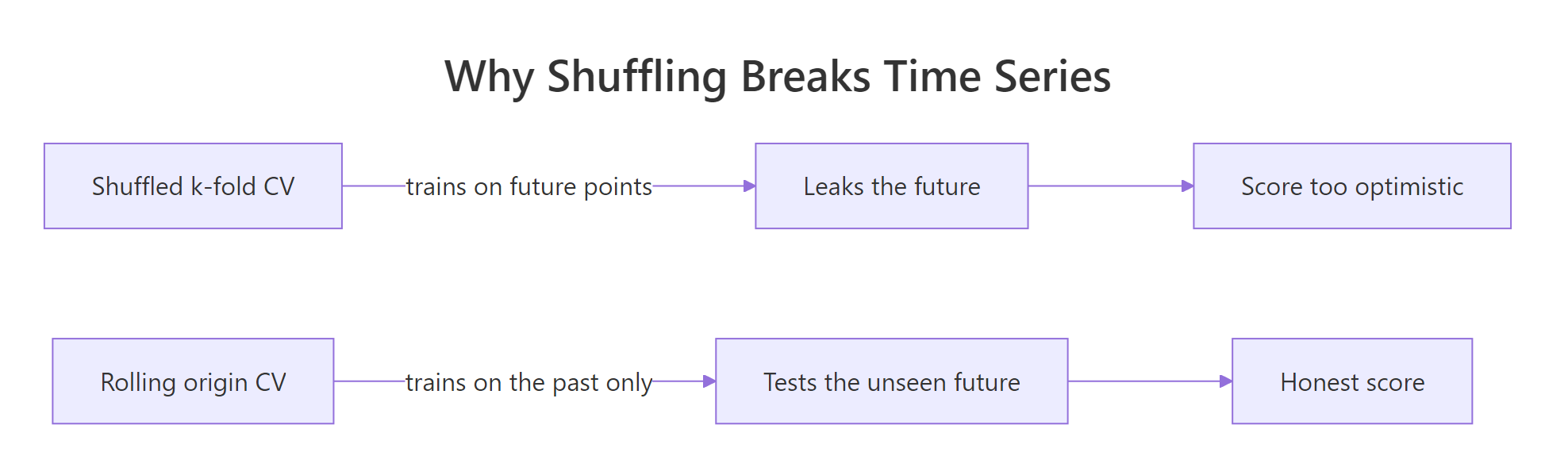
Figure 1: Shuffled cross-validation leaks the future; a rolling origin only ever trains on the past.
Time series cross-validation fixes this by respecting the clock. It only ever tests on points that come after everything it trained on. No forecast is ever allowed to see a value from its own future.
Try it: Swap naive() for meanf() (which forecasts every future point as the average of all past values) and see how the mean forecast scores on the same rolling test.
Click to reveal solution
Explanation: The flat mean forecast scores about 120.6, roughly three and a half times worse than naive. It ignores the trend entirely, so it drifts further below the rising series every year. The rolling test catches that at once.
What is evaluation on a rolling forecast origin?
The idea behind tsCV() has a name: evaluation on a rolling forecasting origin. It sounds fancy, but the recipe is short. Train on the first few points, then forecast the next one and write down the error. Then move the cutoff (the origin) forward by one point, so the training window grows by one, and repeat. By the time you reach the end of the series you have tested the method on hundreds of genuine out-of-sample points, and you average the errors over all of them.

Figure 2: The rolling forecast origin: train, forecast the next point, record the error, then roll forward.
The clearest way to trust tsCV() is to build it yourself on a tiny series and check that you get the same answer. Here is a short series of eight numbers. For each origin t, the naive forecast of the next point is simply the value at t, so the error is the actual next value minus that.
Each stored number is a real one-step error. At origin 2 the forecast for point 3 is the value at point 2, which is 10, and the actual point 3 is 9, so the error is 9 minus 10, or minus 1. We slide the origin forward one point at a time and collect six of these errors, one for each origin from 2 to 7. Now compare this hand-rolled result with tsCV() on the same series.
The two match exactly, which means tsCV() is doing nothing more mysterious than that loop, just faster and for any model you hand it. Notice two details. First, tsCV() returns a time series object, so each error stays lined up with the origin that produced it. Second, both ends are NA. The first origin has too little history for naive() to fit, and the last origin has no future point left to compare against.
The same pattern appears on the real data. Look at the first year of the airline errors we computed earlier.
January 1949 is NA because there was nothing before it to learn from. Every later month except the last holds a genuine one-step forecast error; only two of the 144 months come back missing, January 1949 at the start (no history) and December 1960 at the end (no future month to score against).
tsCV() returns NA at any origin where the model cannot be fit (too little history) or where there is no future observation left to score against. That is why you always average errors with na.rm = TRUE.If you like symbols, here is the same idea in one line. If you prefer code, skip this box, the loop above says everything the formula does.
$$e_{t} = y_{t+1} - \hat{y}_{t+1 \mid t}$$
Where:
- $y_{t+1}$ is the actual next value
- $\hat{y}_{t+1 \mid t}$ is the forecast of that value made using only data up to time $t$
The score most people report is the root mean squared error over all the non-missing errors:
$$\text{RMSE} = \sqrt{\frac{1}{m}\sum_{t} e_{t}^{2}}$$
Where $m$ is the number of errors that are not NA. Smaller is better, and the units are the same as the data, here thousands of passengers.
Try it: Count how many of the 144 months actually received a forecast error, using the errors object from the payoff block.
Click to reveal solution
Explanation: There are 142 scored points. Two of the 144 months are missing: January 1949 (no history, so naive() cannot fit) and December 1960 (no future month to compare). Every other month contributes one honest error to the average.
How do you run time series cross-validation with tsCV()?
You call tsCV() with three main pieces: the series y, a forecastfunction that says how to forecast, and the horizon h. The forecastfunction is the part that trips people up, so let us be precise about its contract. It is a function of two arguments, y and h, and it must return a forecast object (the thing naive(), rwf(), ets() and friends already produce). tsCV() calls it again and again, handing it a longer slice of history each time.
A small helper keeps the scoring readable, since we compute root mean squared error over and over.
rmse() helper with na.rm = TRUE baked in keeps every comparison consistent and saves you from forgetting the missing-value flag, which would otherwise turn your whole score into NA.Here is a question worth asking: why bother with cross-validation at all, when a model already reports its own residuals? Because a model's residuals are measured on the same data it was trained on, so they flatter it. Cross-validation measures error on data the model never saw. Let us put the two side by side for the drift model.
The cross-validated error (33.98) is larger than the in-sample residual error (33.64). The gap is small here because a drift model has only one thing to estimate, but the direction is the rule, not the exception: residuals almost always look better than reality. The more a model bends to fit its training data, the wider this gap grows, which is exactly when you most need an honest number.
Try it: Remove the drift = TRUE argument so rwf() becomes a plain random walk (identical to naive()), and check its cross-validated RMSE.
Click to reveal solution
Explanation: Without drift the score is 33.83, exactly the naive result from the first section. That is a useful sanity check: a random walk with no drift term is the naive forecast, so the two must agree.
How do you compare forecasting models with tsCV()?
This is where cross-validation earns its keep. Put every candidate model through the same rolling test and read the winner straight off the scoreboard. Because tsCV() takes any forecastfunction, you can loop over a list of them. Let us start with three simple benchmarks: the flat mean, the naive forecast, and the seasonal naive forecast (which predicts each month using the same month one year earlier).
Read that carefully, because it contains a surprise. Seasonal naive (36.45) is slightly worse than plain naive (33.83) for one-month-ahead forecasting here. You might have expected the seasonal method to win on such an obviously seasonal series, but a month ago is a closer match to today than a year ago when the series is climbing, because last year's value misses a whole year of growth. The rolling test reports the measured error either way, so it settles the question rather than your intuition about which method should win.
Benchmarks are meant to be beaten. A model that captures both the trend and the yearly season should do far better. A seasonal ARIMA model, sometimes written as ARIMA(0,1,1)(0,1,1) with a period of 12, is the classic choice for this dataset. We wrap it in a forecastfunction and cross-validate it the same way.
The seasonal ARIMA scores about 12.2, roughly a third of the benchmark errors. This block does real work, because tsCV() refits the model at every origin, so give it a few seconds to run. That cost is the whole point: the score is honest precisely because each forecast was made by a model that had never seen the point it was predicting.
Here is the full scoreboard for the four models we have tried.
| Model | What it assumes | Rolling RMSE |
|---|---|---|
| Mean | The series is flat around its average | 120.56 |
| Seasonal naive | This month equals the same month last year | 36.45 |
| Naive | Tomorrow equals today | 33.83 |
| Seasonal ARIMA | Trend plus a yearly season | 12.17 |
ets(y) or auto.arima(y) into a forecastfunction exactly like the ARIMA above, wrapped in forecast(...). They pick their own settings, so they are convenient, but they refit from scratch at every origin and are noticeably slower to cross-validate, so run those comparisons in your own R session when you have time.Try it: Cross-validate naive() and snaive(), then compare their scores directly.
Click to reveal solution
Explanation: Naive (33.83) edges out seasonal naive (36.45) for one-step forecasting on this rising series. The lesson is not that seasonal naive is bad, it is that you should let the rolling test decide rather than assuming.
How do forecast errors grow as the horizon increases?
So far every forecast looked one step ahead. In practice you often need to forecast several steps out, and a fair test should measure how accuracy decays with distance. Set h to a number bigger than 1 and tsCV() returns a matrix instead of a vector: one column per horizon, so column 3 holds every three-step-ahead error.
The result has 144 rows (one per origin) and 12 columns (one per horizon, from one month ahead to twelve). To score each horizon on its own, take the root mean squared error down each column with colMeans().
The error climbs steadily, from about 12 for next month to about 22 a year out. That is the expected shape: the further ahead you forecast, the less certain you are, because more unknown future has to be bridged. A picture makes the trend obvious.
This is a far more useful summary than a single number. If your business only cares about the next quarter, you can read the error for horizons 1 to 3 and ignore the rest. If you must plan a year ahead, you now know the honest uncertainty at twelve months.
snaive() can produce a curve that is nearly flat or even dips at the twelve-month horizon, because the yearly cycle lines the forecast back up with the right season. A smooth, rising curve like the ARIMA one above is the more typical shape.Try it: Read the six-month-ahead error straight from the matrix, using the sixth column of h_errors.
Click to reveal solution
Explanation: The six-month-ahead RMSE is 20.7, which matches the h=6 entry in the horizon table. Picking a single column lets you report accuracy at the exact lead time your decision depends on.
Should you use an expanding or a sliding window?
By default tsCV() uses an expanding window: every training set keeps all the history before the origin, so it grows by one point each step. That is usually what you want. But sometimes the world changes, and old data becomes misleading rather than helpful. For those cases you can pass window = k to use a sliding window that keeps only the most recent k points and forgets everything older.
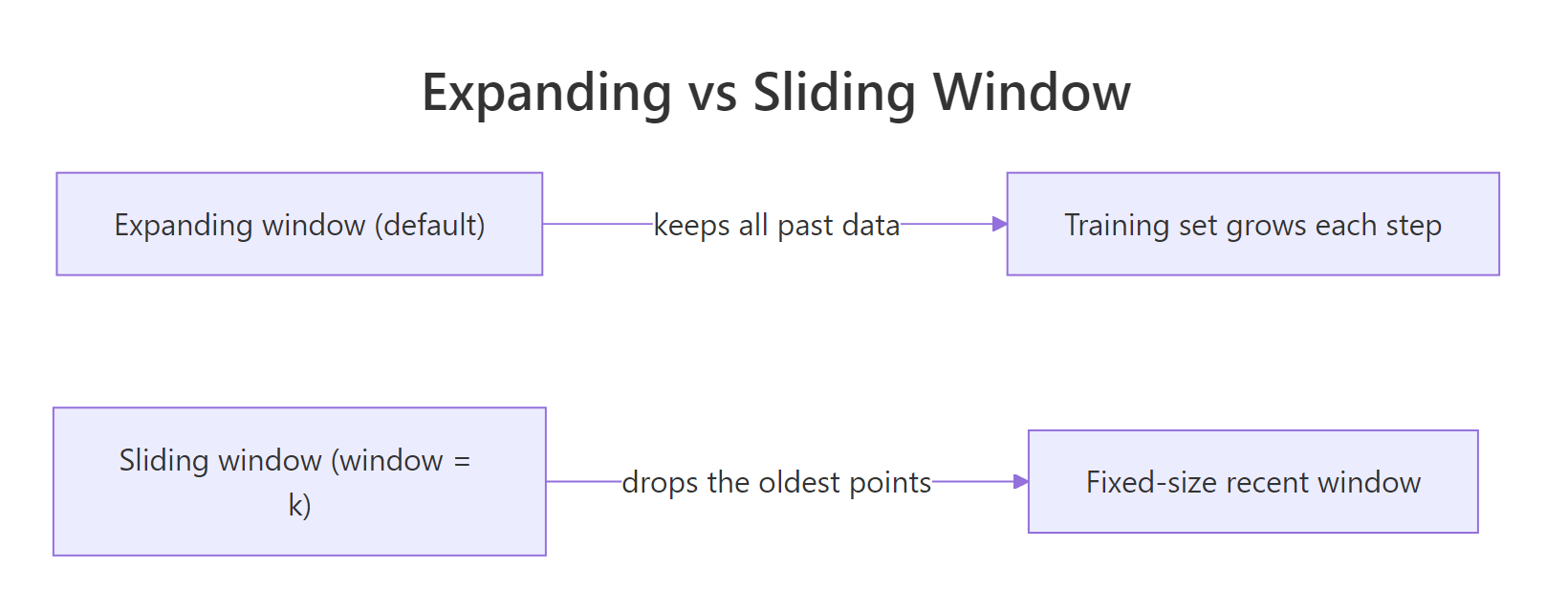
Figure 3: An expanding window keeps all history; a sliding window keeps only the most recent points.
The difference is easiest to see with the mean forecast, which literally averages its training window. On a rising series, an all-history average is held down by the older, lower values, while a recent average tracks the climb far better.
Switching to a two-year sliding window roughly halves the error, from 120.6 to 59.9. The recent-average forecast is still no match for the ARIMA, but the point stands: when the series trends or its behaviour shifts, forgetting stale data can help a lot.
window keeps the model focused on data that still looks like the future you are trying to predict.Try it: A wider window is not automatically better. Change the sliding window from 24 to 48 months and see what happens.
Click to reveal solution
Explanation: A 48-month window scores 86.4, worse than the 24-month window's 59.9. A longer window reaches back to older, lower values and drags the average down again. Window length is a knob to tune, and here 24 months was a better fit than 48.
Complete Example: choose and deploy a model with tsCV()
Let us put the whole workflow together. The goal is a repeatable recipe: cross-validate a shortlist of models, pick the one with the lowest honest error, then refit that winner on all the data and forecast the year ahead. First, the selection step.
The rolling test names the seasonal ARIMA as the clear winner. Now we refit that model on the entire series (cross-validation was only for choosing, the final model should use every observation) and forecast the next twelve months.
The forecast for 1961 climbs into the summer and dips in winter, mirroring the seasonal shape you saw in the very first chart, and it sits above 1960 because the model carries the upward trend forward. Because we chose this model with a rolling test, we can attach an honest error bar to it: about 12 passengers (thousands) for next month, widening toward 22 by the following December.
Practice Exercises
These combine several ideas from the tutorial. Try each one before opening the solution, and use the distinct variable names shown so your code does not overwrite the tutorial objects.
Exercise 1: Pick the better benchmark
Cross-validate the naive and snaive methods on AirPassengers, store their one-step RMSE values in a named vector called my_scores, and print the name of the lower one. Reuse the rmse() helper from earlier.
Click to reveal solution
Explanation: which.min() finds the position of the smallest score, and wrapping it in names() returns the model's label. Naive wins for one-step forecasting here.
Exercise 2: Rank four models in one shot
Write a small helper cv_rmse_of(f) that returns the one-step cross-validated RMSE of a forecastfunction, then use it with sapply() to rank the mean, naive, seasonal naive, and drift methods from best to worst.
Click to reveal solution
Explanation: The helper hides the repetitive tsCV() plumbing so the comparison reads like a ranking. Naive and drift are neck and neck at the top. Seasonal naive trails them, and the flat mean sits far behind.
Exercise 3: Measure what a sliding window buys you
Compare the expanding-window and 24-month sliding-window mean forecasts, and report the percentage improvement the sliding window gives. Store the two scores as my_expanding and my_sliding.
Click to reveal solution
Explanation: The sliding window cuts the error in half, a 50.3 percent improvement, because a recent average tracks the rising series much better than an all-history average.
Frequently Asked Questions (FAQ)
What does tsCV() actually return?
It returns a time series of forecast errors, aligned so each error sits at the origin that produced it. For a one-step forecast (h = 1) you get a vector; for multi-step (h > 1) you get a matrix with one column per horizon. You then reduce those errors to a score yourself, usually with sqrt(mean(e^2, na.rm = TRUE)).
Why are there NA values in the output?
tsCV() inserts NA wherever it cannot produce or score a forecast: at the earliest origins, where there is not enough history to fit the model, and at the very end, where there is no future observation left to compare against. Always pass na.rm = TRUE when averaging, or your score will collapse to NA.
Is tsCV() the same as a train-test split?
A single train-test split checks the model once, on one test window. Time series cross-validation is many train-test splits chained together, moving the cutoff forward one step at a time, so the model is scored on hundreds of out-of-sample points instead of one. That makes the estimate far more stable, especially on shorter series.
Can I use tsCV() with ARIMA, ETS, or my own model?
Yes. Any method works as long as you wrap it in a forecastfunction(y, h) that returns a forecast object. For models that must be fitted first, like ARIMA or ETS, use the pattern function(y, h) forecast(Arima(y, ...), h = h). Be aware that models which refit from scratch at every origin are slower to cross-validate.
Should the final model be trained on all the data?
Yes. Cross-validation is only for choosing between models and estimating their error. Once you have picked a winner, refit it on the entire series so the deployed model uses every observation available, then forecast forward.
How is cross-validation error different from a model's residuals?
Residuals are measured on the same data the model was trained on, so they understate real error. Cross-validation error is measured only on unseen future points, so it is the honest estimate of how the model will perform going forward. The cross-validated number is usually larger, and it is the one to trust.
Summary
Time series cross-validation is the discipline of testing a forecast only on data that comes after everything it trained on, and tsCV() makes it a one-line habit.
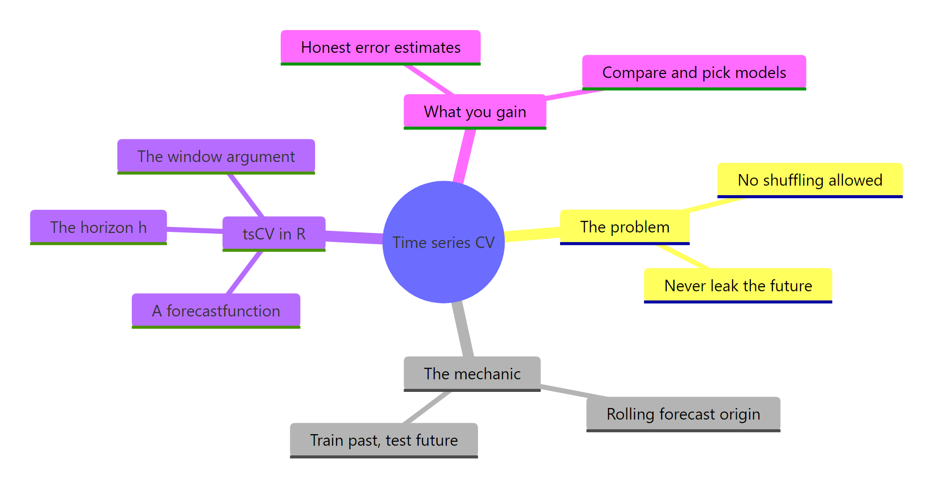
Figure 4: The whole idea of time series cross-validation on one page.
| Idea | What to remember |
|---|---|
| The problem | Shuffled k-fold leaks the future into the test and flatters the model |
| The mechanic | Roll the origin forward: train on the past, test on the next point, repeat |
| The call | tsCV(y, forecastfunction, h) returns a series (or matrix) of out-of-sample errors |
| The forecastfunction | A function of (y, h) that returns a forecast object |
| Scoring | sqrt(mean(e^2, na.rm = TRUE)), always with na.rm = TRUE |
| Comparing models | Rank by cross-validated error, never by in-sample fit |
| Horizons | Set h > 1 to see how error grows with lead time |
| Windows | Default is expanding; use window = k to forget stale data |
| After choosing | Refit the winner on all the data before forecasting |
With this in hand, you can stop guessing which forecast is best and start measuring it, on the only test that matches real life.
References
- Hyndman, R.J. Cross-validation for time series. Hyndsight blog. Link - the short post that introduced the rolling
tsCV()approach, from the author of the forecast package. - Hyndman, R.J., and Athanasopoulos, G. Forecasting: Principles and Practice (3rd ed), Section 5.10: Time series cross-validation. Link - the textbook treatment of the rolling forecast origin, with worked
tsCV()code. - Hyndman, R.J. et al. tsCV() reference, forecast package documentation. Link - the official argument reference for
window,initial, and the multi-horizon matrix return. - Hyndman, R.J., and Athanasopoulos, G. Forecasting: Principles and Practice (3rd ed), Section 5.8: Evaluating point forecast accuracy. Link - explains RMSE, MAE, and the other error measures you reduce the CV errors to.
- Bergmeir, C., and Benitez, J.M. (2012). On the use of cross-validation for time series predictor evaluation. Information Sciences 191, 192-213. Link - the research case for why ordinary k-fold leaks and rolling-origin evaluation is the fix.
- Tashman, L.J. (2000). Out-of-sample tests of forecasting accuracy: an analysis and review. International Journal of Forecasting 16(4), 437-450. Link - the classic review of out-of-sample forecast testing that grounds the whole idea.
Continue Learning
- ARIMA Models in R: Build the seasonal ARIMA that won our rolling test, and understand what its terms mean.
- auto.arima() in R: Let R search for a good ARIMA specification automatically, then cross-validate it the same way.
- ETS Models in R: Learn exponential smoothing, the other workhorse family you can drop straight into
tsCV().