Global Forecasting Models in R: Learn Across Many Series
A global forecasting model is a single model fitted to the stacked history of many time series at once, so that a pattern learned from one series improves the forecast for all the others. It is how the M4 and M5 competitions were won, and it is the only practical option once you have thousands of series to forecast. This page builds one on 152 real Australian retail series, walks into the scaling trap that ruins most pooled models, and then measures whether the global model actually beats one model per series. On this data it does not, and finding out exactly why turns out to be the most useful thing on the page. Every number here was measured, not estimated.
What is a global forecasting model, and how is it different from what you do now?
If you have forecast more than one series before, you have almost certainly written a loop. For each product, each store, each region, you fit a model, produce a forecast, then move on to the next one. That is the local approach, and it is what nearly every forecasting tutorial teaches. A global model reverses it: instead of 500 models that each saw one series, you build one model that saw all 500.
We will work with aus_retail, which ships with the tsibbledata package. It holds monthly retail turnover for every combination of Australian state and retail industry, which is exactly the shape of problem global models were invented for.
Here is what those lines did. aus_retail arrives as a tsibble, a table that knows which column is time and which columns identify each separate series, so as_tibble() strips that wrapper off and leaves us with an ordinary data frame. The state_code vector is a lookup table: writing state_code[State] replaces every long state name with its three-letter code, which keeps the series labels short enough to read. as_date() turns the year-month labels into real dates so lubridate can pull months and years out of them later.
The result is 64,532 monthly observations spread across 152 separate series, each running from April 1982 to December 2018. That is 152 forecasting problems, and 152 is a small number by industrial standards. A supermarket chain forecasts a few hundred thousand.
The single most important fact about these series is that they are not the same size. Some of them are not even close.
group_by() splits the table into one group per series, summarise() collapses each group to a single row holding its length and its average turnover, and arrange() sorts the result so the smallest series float to the top. Stacking the first three rows on top of the last three with bind_rows() gives us both ends of the range in one view.
Read the avg column. Newspaper and book retailing in the Northern Territory averages 2.5 million dollars a month. Food retailing in New South Wales averages 1,653 million. The largest series is roughly 650 times the smallest. Hold on to that number, because it is the single fact that decides whether a global model works or falls over, and we will come back to it in a dedicated section.
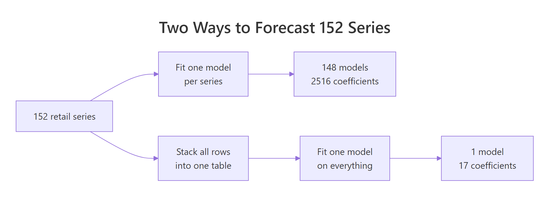
Figure 1: The same 152 series, fitted two ways.
Try it: The block below lists three New South Wales series in ascending order of size. Change it to show the three largest Victorian series instead. You need to change the state code and add a sort.
Click to reveal solution
Explanation: sizes was already sorted ascending by arrange(avg), so head() returned the smallest. Adding arrange(desc(avg)) reverses the order and puts the biggest series first.
Why would a model trained on other retailers' sales help predict yours?
This is the question that decides whether the whole idea is sensible. Why should sales of hardware in South Australia teach a model anything useful about clothing sales in Tasmania? They are different products, different customers, different states.
The answer is that the model is not learning about hardware or clothing. It is learning about shape: the way retail turnover moves from month to month. Let us look at four series drawn from opposite ends of the size range.
Run that and you get a chart with one line soaring near 2,000 and three lines squashed flat along the bottom axis. In dollar terms these series have nothing in common. You cannot even see the shape of the small ones.
Now divide every series by its own long-run average, so each one is expressed as a multiple of its own typical month rather than in dollars.
The four lines now sit on top of each other. All four climb over the decades, all four wobble up and down within each year, and all four spike at the same time of year. The dollar amounts were hiding a common structure that was there the whole time.
That impression deserves a number rather than an eyeball. Below we compute a seasonal index for every series: for each calendar month, how does turnover in that month compare to the average month of the same year?
Walk through the calculation. The first group_by() works within each series and each year, so year_avg becomes the average month of that particular year for that particular series. Dividing an actual month by that average removes both the size of the series and the long-run trend, leaving only the seasonal wobble. The second group_by() then averages that ratio across all the years, giving one index per calendar month per series. Finally we summarise across all 152 series.
Now read the last column, which is the share of series whose index for that month is above 1. In December it is 1.00. Every single one of the 152 series, in every state, in every industry, sells more in December than in its average month, by a median of 38 percent. November is 0.93 and October is 0.79. February is the mirror image: only 2 percent of series are above average.
This is what the literature calls cross-learning, and it has a firmer theoretical footing than you might expect. Montero-Manso and Hyndman proved that for time series forecasting, global methods are not more restrictive than local ones: any set of local models can in principle be matched by a single global model, given enough flexibility. They also showed that the complexity a local approach needs grows with the number of series, while a global model's stays constant. That means a global model can afford to be more complex than any individual series could ever support, and still generalise well.
Try it: The block below summarises December's seasonal index across all 152 series as five quantiles. Change it to look at February instead, and see how the whole distribution shifts below 1.
Click to reveal solution
Explanation: The weakest December series still reaches 1.02, while February's strongest barely scrapes past 1.0 at 1.07. The two months hardly overlap at all. That consistency across 152 independent series is precisely the regularity a pooled model can exploit.
How do you stack many series into one training table?
A model like lm() does not read a time series. It reads a table, one row at a time, and it has no idea the rows are in any order. Before it can forecast anything, the past has to be copied into each row as ordinary columns. If that idea is new to you, the feature engineering tutorial covers it in depth. Here we need just enough of it to make the pooling point.
For each month we build five predictor columns: turnover one, two and three months earlier, and turnover twelve and thirteen months earlier. The first three capture short-run momentum, the last two capture where the series was at this point last year.
The helper deserves a line-by-line reading, because everything downstream rests on it. lg(k) builds a lagged column by gluing k missing values onto the front of the series and dropping k values off the back, which slides every value down by k rows. split() cuts the 152 series apart, lapply() runs the helper on each one separately, and do.call(rbind, ...) stacks the 152 results back into one table. Splitting first is not optional: if you lagged the whole table at once, the last row of one series would leak into the first row of the next.
complete.cases() then drops the first thirteen rows of every series, the ones where the lags do not exist yet. That costs us 1,976 rows and leaves 62,556. Turning month into a factor tells lm() to treat it as twelve separate categories rather than a number where December is twelve times January.
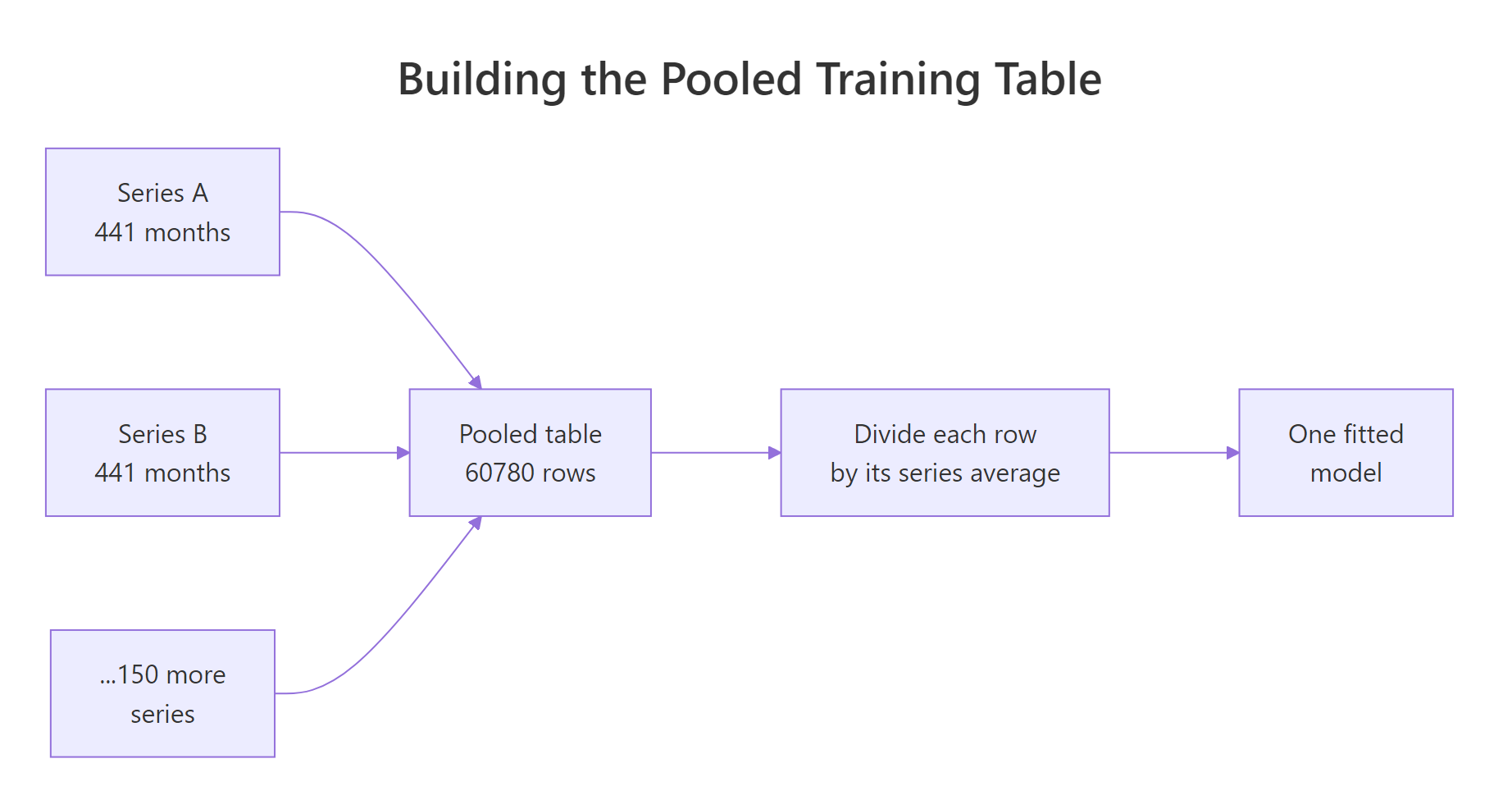
Figure 2: Every series contributes rows to one training table.
Look at the table that came out. It has a series column, but every other column is just a number. Rows from Tasmanian clothing and rows from New South Wales food sit side by side, and nothing marks where one series ends and the next begins. That is the point. To the model this is one dataset of 62,556 examples of the question "given these five recent numbers and this calendar month, what comes next?"
Now we split into a training period and a test period, by date.
Everything up to December 2017 trains the model. All of 2018 is held back. That is 1,776 test points, which is 12 months across 148 series. The count is 148 rather than 152 because four categories, liquor and specialised food retailing in Queensland and Tasmania, stopped being reported before 2018. Real datasets have holes like that, and a global model absorbs them without complaint.
lag1 column literally contains January's value, the model would be shown the answer. Every series must be cut at the same calendar moment.Be clear about what "forecast 2018" means here, because it decides how to read every number on the rest of the page. February 2018's lag1 column holds January 2018's actual turnover, so when we score February we are standing at the end of January, not at the end of 2017. Every prediction below is therefore one month ahead, scored across all twelve months of 2018. That is the standard way to compare models that all use the same lag columns, and it is what keeps the local and global comparison fair.
lag1 and step forward a month at a time (recursive), or fit a separate model per horizon, one that predicts twelve months out directly from the lags you actually have (direct). Errors compound under the recursive strategy, so the numbers get worse the further out you go. Neither strategy changes anything about the pooling decision this page measures, which is why we hold the horizon fixed at one month throughout.Try it: The block below counts how many training rows each series contributes and reports the range. Change it to list the three series with the fewest rows, so you can see which categories are barely represented.
Click to reveal solution
Explanation: Two Tasmanian series contribute only 19 training rows each, against 416 for a full-length series. A local model fitted to 19 rows with 17 parameters to estimate has essentially no chance. The global model simply treats those 19 rows as 19 more examples among 60,780.
Why must you rescale each series before pooling?
Now we fit the first real global model, and it will disappoint us. That is deliberate. The failure is the most valuable thing in this section, because it is the mistake that degrades pooled models in production without ever raising an error, a warning, or a bad-looking summary number.
First we need a way to score a forecast that is fair across series of wildly different sizes. Mean absolute percentage error does that: it converts every miss into a percentage of the actual value, so being 10 million out on a 1,600 million series counts as a small error, and being 10 million out on a 2.5 million series counts as a catastrophe.
MAPE has two known weaknesses worth stating before we lean on it. It is undefined when the actual value is zero, and it penalises over-forecasting more heavily than under-forecasting. Retail turnover in this dataset never comes close to zero, so neither weakness bites here. If your series can hit zero, use MASE or RMSSE instead: both divide your error by the error a seasonal naive forecast would have made on the same series, which puts every series on a comparable footing without dividing by the actual value. RMSSE is the measure the M5 competition scored on.
That is our benchmark. The seasonal naive forecast simply says "this month will be whatever it was twelve months ago", which is the lag12 column we already built. It is wrong by 5.92 percent on average across 2018. Any model that cannot beat 5.92 is not worth deploying.
Now the global model. One call to lm(), one formula, all 60,780 rows.
Seventeen numbers, fitted once, now forecast all 148 series. That is a remarkable reduction in moving parts, and a poor result. It scores 5.73 percent against the seasonal naive's 5.92 percent, an improvement so small it would not survive a different test year.
Something is badly wrong, and averaging hides it. Let us split the series into four groups by size and score each group separately.
scale_of records each series' average turnover during training. cut() with quantile() then chops the series into four equal-sized buckets by that average, and we score each bucket on its own.
The result is stark. On the largest quarter of series the model is off by 2.24 percent, which is genuinely good. On the smallest quarter it is off by 13.19 percent, which is far worse than doing nothing at all. The single average of 5.73 percent describes no actual series. The model is excellent for big retailers and useless for small ones.
The reason is the loss function. lm() chooses its 17 coefficients to minimise the total squared error in dollars, summed over every row of every series:
$$\text{loss} = \sum_{i=1}^{152} \sum_{t} \left( y_{i,t} - \hat{y}_{i,t} \right)^{2}$$
Where:
- $y_{i,t}$ = actual turnover for series $i$ in month $t$, in millions of dollars
- $\hat{y}_{i,t}$ = the model's prediction for that same month
- the inner sum runs over every month of series $i$, the outer over all 152 series
Now put numbers in. A 10 percent miss on New South Wales food retailing is about 165 million, which squared is roughly 27,000. A 10 percent miss on Northern Territory book retailing is 0.25 million, which squared is 0.06. The big series contributes four hundred thousand times more to the total. So whenever a coefficient value that suits the big series conflicts with one that suits the small series, the big series outweighs it four hundred thousand to one, and the fitted coefficients end up describing the big series alone.
The fix follows straight from the diagnosis. If the problem is that series live at different scales, put them all on the same scale. We divide every value in a series, target and lags alike, by that series' average turnover during the training period.
Two details matter here. First, the scale is computed from the training window only. Using the full history including 2018 would leak information about the test period into the features. Second, we scale the target in the training data but not in the test data, because the test target is what we are trying to predict and must stay in its original dollars for scoring. We keep the scale column so we can convert predictions back.
The ACT cafes series now sits around 0.22, meaning that month ran at 22 percent of the series' long-run average. Every series in the table now speaks the same language: multiples of its own typical month.
Note the * test_s$scale on the prediction line. The model returns a forecast in scaled units, so multiplying by the series' own scale converts it back to millions of dollars. Forget that step and every forecast comes out near 1.
Error drops from 5.73 percent to 3.82 percent. Same data, same formula, same 17 coefficients, same lm() call. The only change was the units. Let us confirm the improvement landed where the damage was.
This is the whole lesson in four rows. The smallest series improve from 13.19 percent to 5.95 percent, less than half the error. The largest series get very slightly worse, 2.24 to 2.28, because they no longer monopolise the fit. That is the trade you want: a rounding error of harm to the series that were already fine, in exchange for rescuing the ones that were broken.
It is worth looking at what the model actually learned, because with a linear model you can just read it.
Those six numbers are a compact description of how Australian retail behaves. Last month carries a weight of 0.737 and the same month last year carries 0.840, so the forecast is roughly "where you were last month, corrected by where you were this time last year". The month before last year, lag13, comes in at -0.669, almost cancelling lag12.
That combination is not arbitrary. Adding roughly one unit of lag12 and subtracting roughly one unit of lag13 is the same as adding last year's month-on-month change to this year's level. The model worked out, from data alone, that it should carry over last year's seasonal step rather than last year's level. Classical seasonal ARIMA models encode that exact structure by hand. Here 152 series agreed on it.
Try it: We scaled each series by its mean. The mean is sensitive to a few unusual months, so the median is often a safer choice. Swap mean(y) for median(y) below and see whether it helps.
Click to reveal solution
Explanation: Identical to two decimal places. That is the useful finding: the model is not sensitive to which sensible statistic you scale by, only to whether you scale at all. Mean, median, last value or standard deviation will all rescue you from the 5.73 percent disaster. Pick one, compute it from training data only, and move on.
Does one global model actually beat one model per series?
Most articles on this topic stop here, having shown that a global model works, without ever checking it against the obvious alternative. We are going to check.
The comparison has to be fair, which means changing exactly one thing. Same features, same model family, same training window, same test set. The only difference is whether the rows are pooled or kept apart.
The loop walks the series one at a time, fits lm() to that series alone, and writes its 2018 predictions into the right slots. Notice there is no scaling anywhere in this loop, and it is not an oversight. A model fitted to a single series only ever sees one scale, so dividing that series by a constant would change its coefficients and leave its predictions exactly the same. Scaling is a problem created by pooling, and it exists only for the global model.
Now the scoreboard.
The honest answer is that on this dataset, one model per series wins. 3.58 percent against 3.82 percent. The global model loses by about seven percent in relative terms.
That result is worth sitting with, because it contradicts a great deal of confident writing on this subject. It is also completely unsurprising once you look at what these series are. Every one of them has up to 441 monthly observations, which is 37 years of history. A local model with 17 parameters and 400 rows of clean, strongly seasonal data has everything it needs. There is nothing left for cross-learning to add.
What the global model bought instead was 17 coefficients rather than 2,516. That is a 148-fold reduction in what you have to fit, store, monitor, retrain and debug. Whether 0.24 percentage points of accuracy is worth that trade is a question about your engineering team, not about statistics.
The average also conceals a split decision.
The global model is beaten overall, yet it wins outright on 60 of the 148 series. This is not one approach dominating another; it is two approaches with different failure modes, and the aggregate number picks a winner by a narrow margin.
Try it: The block below finds the three series where the global model beats the local one by the widest margin. Reverse the subtraction to find where local wins biggest instead.
Click to reveal solution
Explanation: Local wins are larger at the top end, 4.61 points against 1.67, which is why local wins the average despite winning fewer series. Series where the local model triumphs tend to have their own idiosyncratic behaviour, exactly the thing a shared set of coefficients cannot represent.
When does the global model win, then?
We have one result on one dataset. That is an anecdote, not a rule. To turn it into a rule we need to work out which property of this data made the local approach win, and then vary that property.
The obvious candidate is history length. The local models had 400 rows each. The global model's advantage is supposed to be that it borrows data from elsewhere, which should matter most when there is little data at home. So let us shorten the history and watch.
The function below repeats the entire comparison using only the most recent N years of training data. Everything else, the test set, the features, the scaling, stays identical.
One line inside that function needs explaining. The local predict() call is wrapped in suppressWarnings() because at two years of history several series have fewer training rows than the model has parameters to estimate, so lm() cannot pin all 17 down and R warns that the prediction comes from a rank-deficient fit. Those warnings are part of the finding, not noise to be hidden: they are R telling you the local approach has run out of data.
Read the two error columns side by side, because the contrast between them is the entire point of this page.
The local column moves a great deal: 5.46 percent with two years of history, falling to 3.58 percent with the full 36. Cut a local model's history and its accuracy falls with it, because 24 rows cannot support 17 parameters.
The global column barely moves at all: 4.05 down to 3.82. Cut every series from 36 years to two and the global model loses almost nothing, because it still has roughly 3,500 training rows, gathered from 148 series at once. The amount of data it learns from barely changed.
The two columns cross somewhere between three and five years. Below that, the global model wins, and at two years it wins by a wide margin, 4.05 against 5.46. Above it, the local model pulls ahead and stays ahead.
The chart shows one steeply falling line and one nearly flat one, crossing near the four-year mark.
This also explains the M5 competition result, where global models swept the leaderboard. Those were daily Walmart sales for individual products, many of them short, and many of them intermittent, meaning most days record a sale of zero. That is the left-hand end of our chart, where the global line sits comfortably below the local one. Australian retail aggregates with 37 years of smooth monthly history are the right-hand end.
Try it: The block below runs the comparison for seven years of history. Change it to 20 years and confirm that the local model's lead widens as history grows.
Click to reveal solution
Explanation: At seven years the local model leads by 0.19 points; at twenty years it leads by 0.31. The gap grows because the local model keeps improving while the global model has already plateaued. It also shows the local model peaking early: 3.51 at twenty years is marginally better than 3.58 with the full 36, since retail behaviour in the 1980s is not very relevant to 2018.
What can a global model do that a local model simply cannot?
Accuracy is not the only axis. There is one thing a global model does that a local model cannot do at all, at any level of accuracy, and for many businesses it is the reason the whole approach exists.
A local model needs your series' history to exist before it can be fitted. If the series is brand new, there is nothing to fit. A global model has no such requirement, because its coefficients came from other series. Forecasting a series that has no history of its own is called the cold-start problem, and it is the one situation where a local model has nothing to offer at all.
We can test that directly. Below we remove 20 series from the training data completely, so the model never sees a single row from them, then ask it to forecast their 2018.
Compare the last two numbers carefully. A model trained on 132 series forecasts 20 completely unseen series at 3.53 percent error. The model that did train on those same 20 series scores 3.54 percent. They are the same to within noise, and the unseen version is fractionally ahead by chance.
The global model gains essentially nothing from having seen your particular series before. Everything it knows about how Australian retail behaves, it learned from the others.
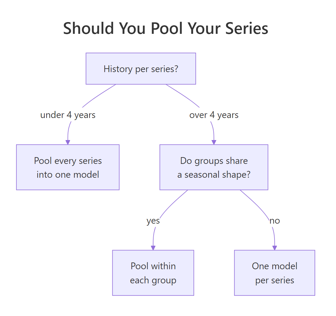
Figure 3: Where each pooling choice makes sense.
The same property has a less glamorous but equally valuable consequence in production. One model means one artefact to version, one training job to schedule, one set of coefficients to review when a forecast goes wrong, and one thing to monitor for drift. Anyone who has maintained a few thousand independently fitted models will recognise why that matters.
Try it: The block below holds out 5 series. Change it to hold out 40, a quarter of the dataset, and see whether cold-start accuracy degrades when the model has fewer series to learn from.
Click to reveal solution
Explanation: Holding out 40 series leaves only 108 to train on, and error rises from 3.58 to 3.74 percent. Some of that is the smaller training set and some is that a different, harder set of series is being scored. Either way the degradation is mild, which is the reassuring result: cold-start forecasting does not collapse when the training pool shrinks by a quarter.
How related do the series have to be?
So far we have treated pooling as a switch with two settings: every series in one model, or every series in its own. It is really a dial. You can pool within groups of similar series, which gives the model more data than a local fit while asking it to describe less variety than a fully global fit.
Our data has an obvious grouping already: the retail industry. Clothing behaves like clothing whichever state it is in. Let us fit one model per industry, pooling the eight states together.
Twenty models, one per industry, each trained on that industry's eight state-level series. Note that we still use the scaled table, because the states differ enormously in size even within a single industry.
Putting all three settings of the dial side by side:
Industry pooling lands at 3.63 percent, within a whisker of the 148-model local approach and clearly ahead of the fully global one, while needing only 20 models. On this dataset that is the best accuracy-per-model trade available.
Why does grouping help here? Because different industries genuinely behave differently, and a single shared set of coefficients has to average over that difference. The try-it below lets you see it directly.
Try it: The block below prints the coefficients that the liquor retailing model learned. Change the industry to "Department stores" and compare the lag1 and lag13 values. They tell two completely different stories.
Click to reveal solution
Explanation: Liquor retailing leans hard on last month, 0.675, and cancels most of lag12 with lag13 at -0.638. Department stores almost ignore last month, 0.111, and barely use lag13 at all, -0.042. Department stores are so violently seasonal that December tells you nothing about January; last year's same month is nearly the whole signal. A fully global model has to split the difference between these two behaviours, and serves neither industry as well as its own model does.
Complete Example: the whole pipeline in one place
Everything above, condensed. This block assumes the objects built earlier in the page still exist, prints the summary of what was fitted, and then shows six months of the 2018 forecast for one series so you can see the actual numbers rather than an error statistic.
Those forecasts for a mid-sized Tasmanian clothing series came from a model that also forecasts New South Wales food retailing, a series 80 times larger, using the same 17 numbers. February is the worst month of the six, forecast at 15.7 against an actual 20.2, which is the model applying the average February dip to a series whose dip is shallower than most. That is the cost of sharing coefficients, visible in a single row.
Practice Exercises
Exercise 1: Give the global model per-industry seasonality
The fully global model applies one shared set of month effects to all 152 series, which we saw is a poor fit for department stores. Add an interaction between month and Industry to the formula so the model can learn a separate seasonal pattern per industry, while still being one model. Fit it on train_s, predict on test_s, and report both the coefficient count and the MAPE against the plain global model's 3.82 percent.
Click to reveal solution
Explanation: The model improves from 3.82 to 3.77 percent, and it is still one model, one training run, one artefact. It now carries 245 coefficients instead of 17, which is a lot more than the global model had but still an order of magnitude fewer than the 2,516 the local approach needed. This is the Montero-Manso and Hyndman argument made concrete: a global model can afford extra complexity because it has 60,780 rows to support it, where a single series had only 400.
Exercise 2: Pool by state instead of by industry
We pooled by industry and got 3.63 percent from 20 models. State is the other obvious grouping in this data. Fit one model per state, pooling all industries within each state, and compare. The state code is the part of the series string before the " / ", which sub(" /.*$", "", series) will extract. Predict on the scaled test table and report the MAPE.
Click to reveal solution
Explanation: State pooling scores 3.78 percent, barely better than the fully global 3.82 and clearly worse than industry pooling's 3.63. The lesson generalises: group by whatever drives the dynamics, not by whatever labels happen to be in your data. What a shop sells determines its seasonal shape. Which state it sits in mostly determines its size, and we already removed size by scaling.
Exercise 3: Scale from recent history instead of all of it
We scaled each series by its mean over the entire training window, 1982 to 2017. For a series that has tripled since 1982, that mean describes a level the series left behind decades ago. Recompute the scale using only 2016 and 2017, refit the global model on the newly scaled data, and see whether a more current scale helps.
Click to reveal solution
Explanation: A marginal improvement, 3.80 against 3.82. The reason the gain is small is that scaling is a per-series constant, and a linear model largely absorbs a constant. The reason to prefer the recent window anyway is operational: in production you refit periodically and your scale should track the series' current level, otherwise a series that has doubled will feed the model lag values near 2.0 that it has rarely seen in training. Try this exercise again with a nonlinear learner and the gap widens considerably.
Frequently Asked Questions
Does this replace ARIMA and ETS? No. Those are local models by construction, and this page just showed a local approach winning on long, clean, seasonal series. fable's model() function fits one model per key in a tsibble, which is the local approach done well, and for a few hundred long series it remains an excellent default. Global models earn their place when series are numerous and short, or when new ones keep appearing.
Why use lm() when everyone uses LightGBM? Because the pooling decision is what this page is about, and a linear model lets you read the shared coefficients directly and see what cross-learning actually learned. In production a global model is usually a gradient boosted tree, which handles the nonlinearity and the interactions that our linear formula cannot. The pooling, scaling and evaluation logic is identical either way. The gradient boosting tutorial covers the learner side.
How many series do I need before pooling helps? There is no threshold, because it depends on length as much as count. The useful question is the one the crossover table answers: how much history does each series have? Below roughly three or four years of monthly data, our global model won even with 148 series. The two quantities trade against each other, so run the compare_history() experiment on your own data rather than trusting a rule of thumb.
Do I still need to scale if I use trees? More than ever. A linear model partly absorbs scale differences through its coefficients. A tree splits on raw thresholds, so a rule like "if lag1 is above 300" is meaningless for a series that never exceeds 5. Trees cannot extrapolate beyond the range they were trained on either, so an unscaled global tree caps its forecast for your largest series at the highest value it happened to see during training.
How do I forecast twelve months ahead instead of one? Pick recursive or direct. Recursive means predicting January, treating that prediction as January's actual value so it becomes February's lag1, and stepping forward: simple, one model, but each month's error feeds the next. Direct means fitting a separate model per horizon, each using only lags that are genuinely available at the forecast origin, so a twelve-month model would drop lag1, lag2 and lag3 and lean on lag12 and lag13: more models to maintain, no error compounding. Direct tends to win at long horizons; the pooling and scaling logic on this page is unchanged either way.
Does a global model give me prediction intervals? lm() will produce them with predict(..., interval = "prediction"), but they assume constant variance across all pooled rows, which is unlikely to hold even after scaling. For pooled models, empirical intervals from held-out residuals are the safer route, and conformal prediction is the principled version of that idea.
Summary
| Question | Answer from this page |
|---|---|
| What is a global model? | One model fitted to the stacked rows of many series, storing one shared set of parameters |
| What makes pooling work? | Shared shape. All 152 series peak in December, by a median of 38 percent |
| What breaks it? | Unscaled pooling. Error on the smallest quarter of series was 13.19 percent, against 2.24 on the largest |
| How do you fix it? | Divide each series by its own training mean, then multiply predictions back. Error fell from 5.73 to 3.82 percent |
| Did global beat local here? | No. 3.82 against 3.58 percent, though it won on 60 of 148 series with 17 coefficients instead of 2,516 |
| When does global win? | When series are short. Below about four years of history, global led; at two years it led by 1.41 points |
| What is global-only? | Forecasting a series that was never in training. Cold-start scored 3.53 percent, matching the model that had seen it |
| What is the best setting? | Often neither extreme. Pooling by industry gave 3.63 percent from 20 models |
References
- Montero-Manso, P. and Hyndman, R.J. Principles and Algorithms for Forecasting Groups of Time Series: Locality and Globality. International Journal of Forecasting (2021). Link
- Hyndman, R.J. and Athanasopoulos, G. Forecasting: Principles and Practice, 3rd edition. Chapter on judgmental and many-series forecasting. Link
- Makridakis, S., Spiliotis, E. and Assimakopoulos, V. The M5 Accuracy competition: Results, findings and conclusions. International Journal of Forecasting (2022). Link
- Januschowski, T. et al. Criteria for classifying forecasting methods. International Journal of Forecasting (2020), the paper that formalised the local versus global distinction. Link
- Hewamalage, H., Bergmeir, C. and Bandara, K. Global Models for Time Series Forecasting: A Simulation Study. Pattern Recognition (2022). Link
- tsibbledata package reference,
aus_retaildataset documentation. Link - fable package documentation, fitting models across many series with
model(). Link - R Core Team. An Introduction to R, section on statistical models and formulas. Link
Continue Learning
- Feature Engineering for Time Series Forecasting in R covers the lag, rolling, calendar and Fourier features that fill a pooled table, and the leakage traps that come with them.
- Gradient Boosting for Time Series in R: xgboost vs the Classics swaps the linear learner used here for boosted trees, and shows why trees cannot extrapolate a trend.
- Time Series Cross Validation in R replaces the single 2018 holdout used on this page with a rolling origin, which is how you should evaluate any of these models before deploying them.