Forecast Accuracy in R: MAE, RMSE, MAPE, and MASE
Forecast accuracy is how close your predictions come to what actually happened. In R you measure it with four standard metrics, MAE, RMSE, MAPE, and MASE, and the accuracy() function in the forecast package reports all of them from a single call.
What is forecast error, and why measure accuracy?
A forecast is only useful if you know how wrong it usually is. Every accuracy metric on this page starts from one simple number: the forecast error, which is the actual value minus the value you predicted, computed for each time period. Once you are comfortable with that single quantity, every metric that follows is just a different way of averaging it.
Let's make it concrete. Suppose you forecast weekly demand for a product and, after six weeks, you line up what you predicted against what actually sold. Subtracting one from the other gives you the error for each week.
We stored six weeks of actual sales and the six matching forecasts, then subtracted the forecasts from the actuals. R does this element by element, so week 1 gives 112 minus 120 = -8, week 2 gives 118 minus 115 = 3, and so on down the vector.
A negative error means the forecast was too high (we predicted 120 but only sold 112). A positive error means it was too low. No single week tells you how good the forecast is overall, which is exactly why we need to boil these six numbers down to one.
It helps to see the errors next to the numbers they came from. The absolute error, the size of the miss regardless of direction, is what most metrics actually work with.
The abs_error column drops the sign, so an 8-unit miss below and an 8-unit miss above count the same. Summing or averaging that column is the foundation of every metric ahead.
One more habit before the metrics: you should always score a forecast on data the model has not seen. In practice you hold back the most recent slice of history as a test set, forecast it, then compare against what really happened. Grading a model on the same data it learned from flatters it.
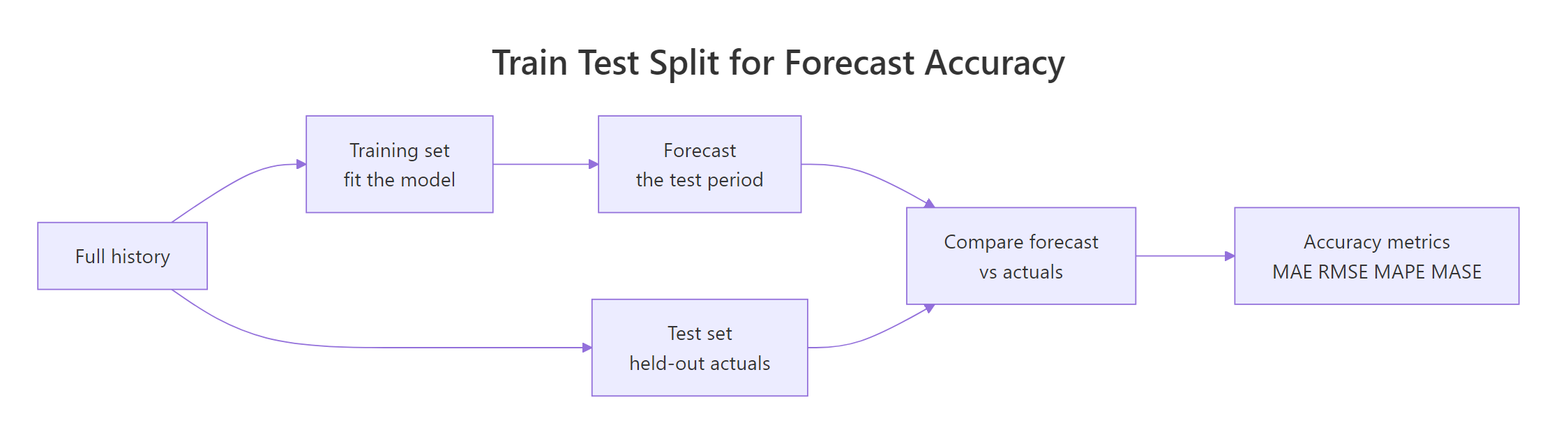
Figure 1: Hold out the most recent data as a test set, forecast it, then compare against the actuals to score accuracy.
Try it: Compute the forecast error for a new three-week run of actuals and forecasts.
Click to reveal solution
Explanation: Subtraction is vectorised, so R pairs each actual with its forecast automatically. Week 1 beat its forecast by 2, week 2 fell short by 3, week 3 beat it by 3.
How do MAE and RMSE measure the size of errors?
The error vector has six numbers and mixed signs. To report a single "typical error", you have to average them, and the first question is what to do about the signs. If you just averaged the raw errors, positives and negatives would cancel and a wildly wrong forecast could look perfect. So both workhorse metrics remove the sign first.
Mean Absolute Error (MAE) takes the absolute value of each error, then averages. Root Mean Squared Error (RMSE) squares each error (which also removes the sign), averages, then takes the square root to get back to the original units.
In symbols, with $n$ errors:
$$\text{MAE} = \frac{1}{n}\sum_{t=1}^{n} |e_t| \qquad \text{RMSE} = \sqrt{\frac{1}{n}\sum_{t=1}^{n} e_t^2}$$
Where:
- $e_t$ = the forecast error in period $t$ (actual minus forecast)
- $n$ = the number of periods you are scoring
- $|e_t|$ = the absolute value, or size, of that error
If the notation is not your thing, skip it: the two lines of code below say exactly the same thing.
Both are a one-liner in R. We reuse the error vector from the last section, so there is nothing new to set up.
The first line turns -8 3 4 -4 3 -5 into the sizes 8 3 4 4 3 5 and averages them to 4.5. The second squares each error, averages, then square-roots. On average this forecast misses by about 4.5 units (MAE), and RMSE is a touch higher at 4.81.
They are close here because no single week is dramatically worse than the others. When RMSE and MAE diverge, that gap is telling you something, which is the next thing to see.
RMSE and MAE actually answer slightly different questions. Because RMSE squares the errors before averaging, one big miss counts far more than several small ones. Watch what happens to two error patterns that share the identical MAE.
Both error vectors average to an absolute error of 2, so their MAE is identical. But the spiky vector concentrates all its error in one week, and squaring 12 blows it up, so its RMSE is 4.9 versus 2.0 for the steady vector.
That is the core difference between the two. MAE weights every unit of error equally. RMSE weights larger errors more heavily, because squaring makes big misses count for more. If a single catastrophic forecast hurts you far more than several small ones (think of an inventory stockout), prefer RMSE. If all errors hurt in proportion to their size, MAE is the more honest summary.
Try it: Compute the MAE and RMSE for a set of four errors that includes two larger misses.
Click to reveal solution
Explanation: Same recipe as before. The larger errors (6 and -6) get squared, so they pull RMSE above MAE.
How does MAPE turn errors into a percentage?
MAE and RMSE are in the units of your data. That is fine until someone asks "is a miss of 4.5 good?" You cannot answer without knowing the scale. Being off by 4.5 units on a base of 5 is terrible; on a base of 5,000 it is excellent. Mean Absolute Percentage Error (MAPE) fixes this by expressing each error as a percentage of the actual value, then averaging.
$$\text{MAPE} = \frac{100}{n}\sum_{t=1}^{n} \left| \frac{e_t}{y_t} \right|$$
Where $y_t$ is the actual value in period $t$ and $e_t$ is its forecast error.
For our demand example, we divide each error by the actual sales that week, then average.
Each weekly error is divided by that week's actual, turned into a size with abs(), averaged, and multiplied by 100 to read as a percentage. On average the forecast is off by about 3.7 percent. That number means the same thing whether you sell hundreds or millions of units, which is why it is the metric executives reach for.
MAPE has one serious weakness, though. Because it divides by the actual value, an actual of zero breaks it completely.
The fourth actual is 0. Dividing that week's error by zero gives infinity, and a single Inf makes the whole average Inf. Any series that can hit zero, such as intermittent demand, rainfall, or defect counts, can make MAPE undefined or absurdly large.
MAPE is also asymmetric: it penalises a forecast that is too high differently from one that is too low, because a percentage error is bounded below by zero but unbounded above. Use it for strictly positive series that stay comfortably above zero, like the airline data later in this tutorial, and reach for another metric otherwise.
Try it: Compute the MAPE for three actuals and their forecasts, rounded to two decimals.
Click to reveal solution
Explanation: Each error is divided by its own actual, turned into a size, averaged, and scaled to a percentage. The forecasts are off by about 5.3 percent on average.
Why does MASE let you compare forecasts across different series?
Here is a problem none of the previous metrics solve. Suppose you forecast daily revenue in dollars and daily website visits as a count, and you want to know which forecast is better in a like-for-like way. MAE and RMSE are in different units, so you cannot compare them. MAPE is comparable in principle but breaks near zero. Mean Absolute Scaled Error (MASE) was designed for exactly this.
The idea is to report your error relative to a dead-simple benchmark instead of on its own. The benchmark is the naive forecast, which just predicts that each value equals the previous one. MASE divides your model's MAE by the MAE that naive forecast would have made on the training data. The result is a pure ratio with no units.
$$\text{MASE} = \frac{\text{MAE of your forecast}}{\text{MAE of a naive forecast on the training data}}$$
The denominator, the naive benchmark's error, is just the average absolute one-step change in the training series.
Say your model's MAE on the test set is the 4.5 we computed earlier, and here is the training history the model learned from. We compute the benchmark from that training data, then form the ratio.
diff(train) gives the week-to-week changes (4 -6 12 5 5 -2), and their average absolute size is 5.67. Dividing our model's MAE of 4.5 by that benchmark gives a MASE of 0.79.
Read MASE against the number 1. A value below 1 means your forecast beats the naive "tomorrow equals today" benchmark; above 1 means it is worse than that trivial rule and you should go back to the drawing board. Our 0.79 says the model's errors are about 79 percent the size of the naive benchmark's, a modest but real improvement. Because it is a unitless ratio, you can average MASE across a dollar series and a visits series and compare them directly.
Try it: Compute MASE by hand from a training history and a model's test-set errors.
Click to reveal solution
Explanation: The model's MAE is 2 and the naive benchmark's MAE is 3, so the ratio is 0.667. Below 1, so the forecast beats naive.
How do you compute every metric at once with accuracy()?
Computing each metric by hand is great for understanding, but you would not want to do it every time. The forecast package bundles all of them into one function, accuracy(). You hand it a forecast object and the actual test values, and it returns a table with ME, RMSE, MAE, MPE, MAPE, MASE, and a couple of extras, split into a training-set row and a test-set row.
Let's do it properly on real data. AirPassengers is a built-in monthly series of airline passengers from 1949 to 1960. We train on everything up to the end of 1959 and hold out 1960 as the test set. The window() function slices a time series by date.
We split the series, fit an exponential smoothing model with ets(), forecast the 12 held-out months, and pass the forecast plus the true 1960 values to accuracy(). The Training set row scores the fit on data the model learned from; the Test set row scores it on the held-out year the model never saw.
Always read the Test set row, because the training row flatters the model. On unseen 1960 data the forecast is off by about 23 passengers on average (MAE), 27 in RMSE terms, and 4.7 percent (MAPE). The Test-set MASE of 0.749 is the headline: below 1, so the model comfortably beats a naive benchmark. The mean error (ME) of +12 tells you the model slightly under-forecasts the fast-growing 1960 traffic. ME and MPE (its percentage version) keep the sign of the error rather than removing it, so unlike the size metrics they measure directional bias, whether the forecast tends to run high or low, not how big the misses are.
Try it: Build a plain naive forecast of 1960 and pull its Test-set MAPE from the accuracy table.
Click to reveal solution
Explanation: The naive forecast's MAPE of 14.3 percent is far worse than the ETS model's 4.7 percent, because naive ignores both the upward trend and the seasonality in the data.
Which forecast accuracy metric should you use?
There is no single best metric; the right choice depends on the question you are answering. Here is how the four compare on the things that usually decide it.
| Metric | Units | Robust to outliers | Handles zeros | Compare across series | Reach for it when |
|---|---|---|---|---|---|
| MAE | Data's own units | Yes | Yes | No | You want a plain, robust average error |
| RMSE | Data's own units | No, punishes spikes | Yes | No | Large single misses are especially costly |
| MAPE | Percentage | Somewhat | No, breaks at zero | Loosely | You need a scale-free number on positive data |
| MASE | Unitless ratio | Yes | Yes | Yes | You compare forecasts across different series |
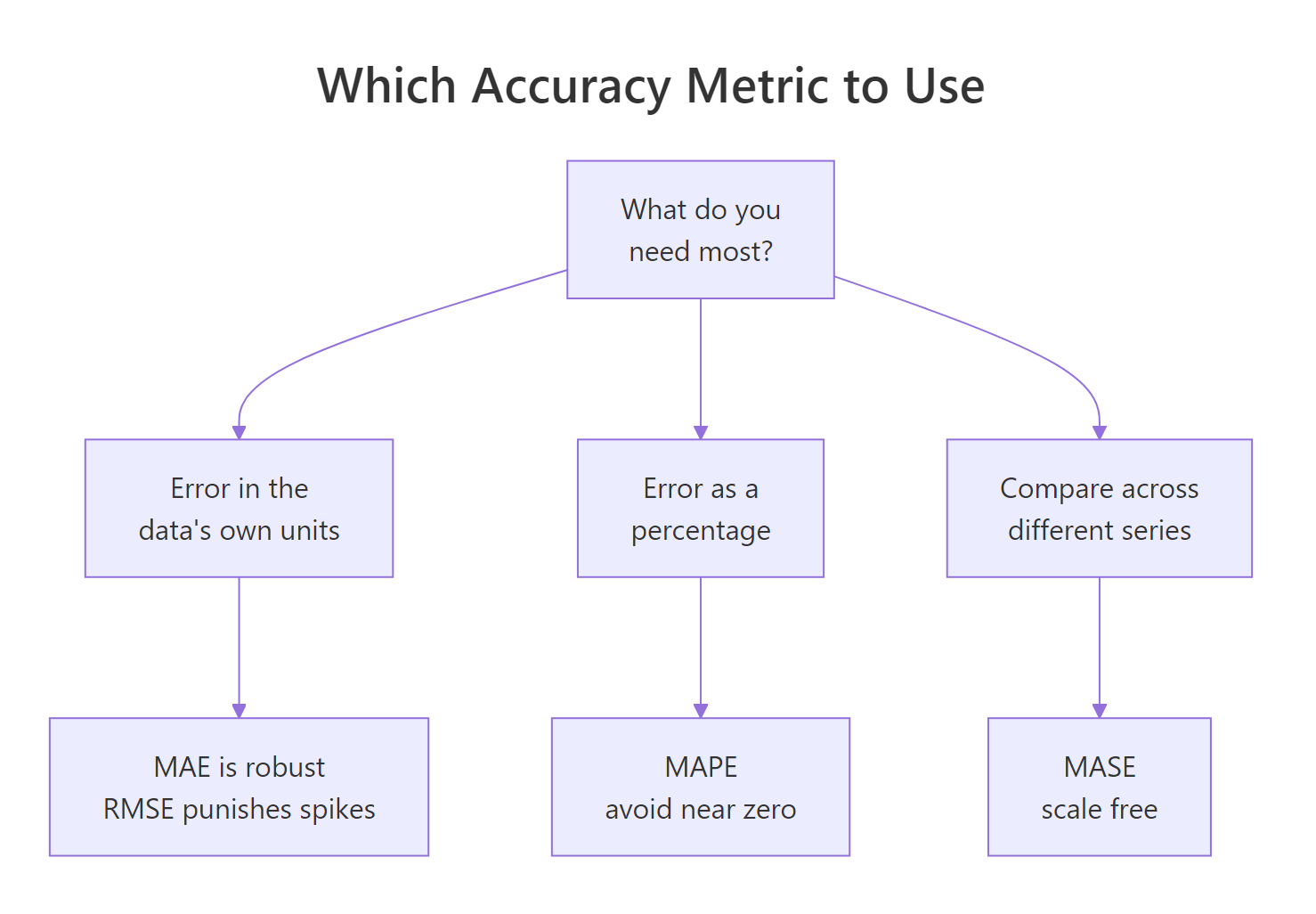
Figure 2: Pick the metric that matches what you care about most.
In day-to-day work it helps to have the scale metrics in one place. This small helper returns MAE, RMSE, and MAPE for any pair of actuals and forecasts, so you never retype the recipe.
The function computes the error inside, then returns the three metrics as a named vector. Calling it on our original demand example reproduces the numbers we found by hand earlier. Wrapping the recipe like this gives you consistent output every time and makes model comparisons a single line.
Try it: Use forecast_metrics() to score two competing forecasts and see which one wins.
Click to reveal solution
Explanation: Forecast A wins on all three metrics; its RMSE of 1.0 is well below B's 1.673, so A is the one to ship.
Complete Example
Let's put the whole workflow together the way you would in practice: split the data, fit a model, forecast the holdout, and compare it against a benchmark to decide whether the model is worth shipping. We already have the ETS forecast fc and the held-out test_ap from earlier. The natural benchmark for a monthly, seasonal series is the seasonal naive forecast, snaive(), which predicts that each month equals the same month one year earlier.
We build the seasonal-naive benchmark, pull the Test-set row for both forecasts, and stack them so every metric lines up side by side.
The ETS model wins on every metric: about half the RMSE and MAE, less than half the MAPE, and a MASE of 0.749 versus 1.571. The benchmark's MASE above 1 shows that even a seasonal rule is beaten here, and the ETS MASE below 1 confirms the model adds real value. This is a clear decision: ship the ETS forecast.
A picture makes the win obvious. autoplot() draws the forecast with its uncertainty bands, and autolayer() overlays what actually happened in 1960.
The shaded fan is the ETS forecast and its uncertainty; the overlaid line is the real 1960 data. The actuals sit inside the forecast band and hug the central line, which is the visual version of that low test-set MASE. Seeing the forecast track the holdout is the final confirmation before you trust it going forward.
Practice Exercises
Time to combine what you have learned. Each exercise runs in the same session as the tutorial, so the functions and data above are still available. Use fresh variable names so you do not overwrite them.
Exercise 1: Pick the better model and explain the disagreement
You forecast a five-period series with two models. Compute the MAE and RMSE of each, decide which model you would ship, and note why RMSE could rank two models differently from MAE.
Click to reveal solution
Explanation: Model A wins on both metrics. Its errors are small and even, so its MAE (2.2) and RMSE (2.236) are almost identical. Model B has larger, more variable errors, so its RMSE (6.372) pulls further above its MAE (6.2). The general lesson: whenever one model has a single large miss, its RMSE climbs faster than its MAE, so the two metrics can disagree about which model is worse.
Exercise 2: Compute MASE from scratch on a train/test split
Given a training history, a short test set, and your forecast for it, compute MASE by hand: scale your test MAE by the training naive benchmark. Is the forecast better than naive?
Click to reveal solution
Explanation: The training series rises fairly steadily, so its average one-step change (the benchmark) is about 1.71. Your forecast's test MAE is 1.0, giving a MASE of 0.583. Below 1, so the forecast beats the naive benchmark.
Exercise 3: Bake off ETS against auto.arima with accuracy()
Using the same AirPassengers train/test split from the tutorial, fit an automatic ARIMA model, forecast 1960, and compare it to the ETS forecast on the four test-set metrics. Which model would you pick by MASE?
Click to reveal solution
Explanation: auto.arima() searches ARIMA orders automatically and, on this holdout, edges out ETS on every metric, with a lower MASE (0.608 versus 0.749). By MASE you would ship the ARIMA model, though both comfortably beat a naive benchmark. The workflow is the point: pick a metric, then let the held-out numbers choose the model.
Frequently asked questions
Which forecast accuracy metric should I use?
There is no single best one. Start with MAE or RMSE to see the error in your data's own units (use RMSE if a rare large miss is especially costly), and add MASE so you know whether the model actually beats a naive benchmark. Reach for MAPE only when you need a percentage and every actual value stays comfortably above zero. Reporting one scale metric plus MASE covers most decisions.
Why is my MAPE infinite (Inf) or extremely large?
MAPE divides each error by the actual value, so any period where the actual is exactly zero produces a division by zero, and a single Inf makes the whole average Inf. Actuals close to zero cause the same problem to a lesser degree, inflating the score without any real change in forecast quality. On data that can hit zero, such as intermittent demand or counts, use MAE or MASE instead.
What counts as a good MASE or RMSE value?
RMSE and MAE have no universal "good" value: a MAE of 5 is excellent on sales in the thousands and terrible on sales in single digits, so you can only judge them relative to the scale of your data or a benchmark. MASE is easier to read because it is scaled: below 1 means your forecast beats a naive "no change" forecast, exactly 1 ties it, and above 1 is worse than doing nothing clever. That is why MASE is the metric to lean on when you want an absolute sense of "is this any good".
What is the difference between MAE and RMSE?
Both remove the sign of each error and report a typical error size in the data's units, but they average differently. MAE averages the absolute errors, so every unit of error counts equally. RMSE squares the errors before averaging, which makes a few large misses count for much more, so RMSE is always at least as large as MAE and the gap between them widens as your errors become more uneven.
Do I need the forecast package to measure accuracy?
No. All four metrics are short one-liners in base R, exactly as computed by hand earlier on this page, so you can score any pair of actuals and forecasts without extra packages. The accuracy() function in the forecast package is a convenience: it computes them all at once from a forecast object and neatly splits the results into a training-set row and a test-set row.
Summary
Forecast accuracy comes down to summarising the forecast error in the way that best fits your decision. Here is the cheat sheet.
| Metric | In plain words | Units | Best for | Watch out |
|---|---|---|---|---|
| MAE | Average size of the errors | Data's units | A robust, everyday error measure | Cannot compare across series |
| RMSE | Like MAE but squares first | Data's units | When big single misses are costly | Sensitive to outliers |
| MAPE | Average error as a percentage | Percent | Scale-free reporting on positive data | Undefined at zero, asymmetric |
| MASE | Error relative to a naive benchmark | Unitless | Comparing across different series | Needs a training series to scale |
The takeaways in one glance:
- Every metric is a summary of the error vector (actual minus forecast); they differ only in how they average it.
- MAE and RMSE live in your data's units, and RMSE punishes large single misses harder.
- MAPE reads as a percentage but breaks on zero or near-zero actuals.
- MASE is the only unitless, cross-series metric; below 1 beats a naive forecast.
accuracy()in the forecast package returns them all at once, and you should always read the Test set row.
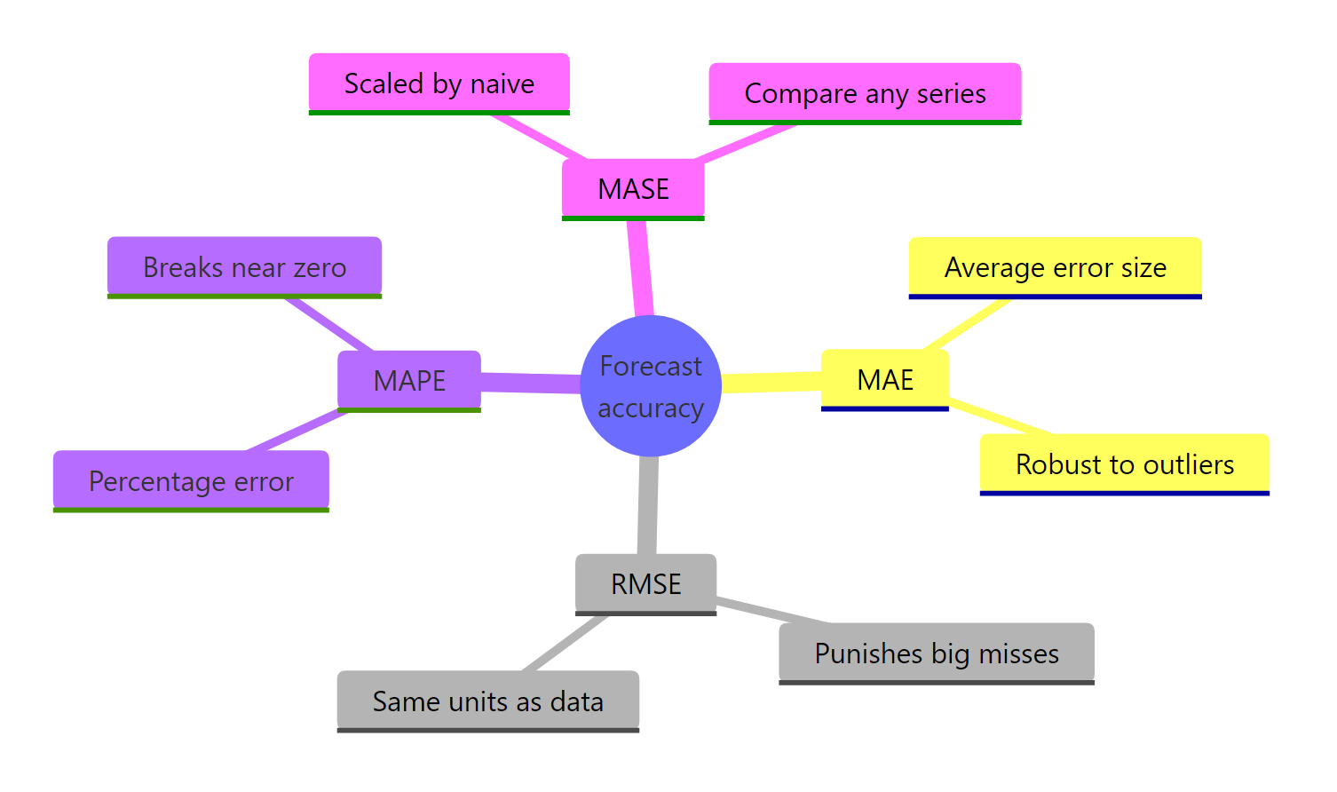
Figure 3: The four accuracy metrics and what each one is good for.
References
- Hyndman, R.J. & Athanasopoulos, G. - Forecasting: Principles and Practice (3rd ed), "Evaluating forecast accuracy". Link
- Hyndman, R.J. & Koehler, A.B. (2006) - "Another look at measures of forecast accuracy", International Journal of Forecasting 22(4). Link
- forecast package -
accuracy()function reference. Link - Hyndman, R.J. - "Errors on percentage errors", on the pitfalls of MAPE. Link
- forecast package on CRAN. Link
- R documentation - the
AirPassengersdataset. Link
Continue Learning
- ETS Models in R - fit the exponential smoothing models whose forecasts you just scored.
- auto.arima() in R - the automatic ARIMA search used in the final exercise.
- Choosing a Forecasting Model in R - use these accuracy metrics to select between competing models.