Gradient Boosting for Time Series in R: xgboost vs the Classics
Gradient boosting for time series means rewriting your series as an ordinary table of lagged columns, then training a long chain of small decision trees where each one corrects the mistakes the previous ones left behind. It is the method that swept the M5 retail forecasting competition, and it also fails on trending data in one specific way that most tutorials never show you. This page builds the boosting loop from scratch so you can watch it work, walks straight into that failure, fixes it, then scores the result honestly against ETS and ARIMA on the same data. Every number on this page was measured, not estimated.
Why can't you hand a time series straight to xgboost?
ARIMA and exponential smoothing take the observations in order, one after another, and that order is part of what they model. A decision tree works on a table instead. Here is everything a regression tree does: it asks a chain of yes/no questions about the columns of one row, such as "is this row's value from a year ago above 300?", and each answer sends the row further down the tree until it arrives at a leaf. The leaf returns the average of all the training rows that ended up there. Nothing in that procedure looks at row order, so shuffling the rows produces the identical model. Before boosting can forecast anything, the past has to be copied into each row as ordinary columns.
We will work with AirPassengers, a monthly count of international airline passengers from 1949 to 1960 that ships with R. It has a strong upward trend and a seasonal pattern that grows with the level, which makes it the ideal series for this tutorial: it is exactly the shape that breaks naive tree-based forecasting.
Read down any column and the numbers climb steadily year after year. Read across any row and you see the same summer peak every year, with July and August far above February. Those two facts, the trend and the season, are the whole story of this page.
The rpart package gives us decision trees, and ggplot2 will draw one chart near the end. We load both now because they persist for the rest of the page.
Now the reframing. For each month we build four columns: the value from twelve months ago, the value from twenty-four months ago, which calendar month it is, and a counter for how far into the series we are.
Each lag column is built by gluing a block of NA values onto the front of the series and chopping the same number off the back. For lag12, twelve NA values go in front, then the original values from position 1 up to position n - 12. That shift is what slides January 1950's value into January 1951's row.
The first rows are mostly NA because there is no "twelve months ago" for 1949. Look further down and the columns fill in.
Row 25 is January 1951. Its y is 145, the actual count for that month. Its lag12 is 115, which is January 1950. Its lag24 is 112, which is January 1949. Look back at the printed series and you will find those exact numbers in the January column. The row now carries its own history.
The month column is stored as a plain number from 1 to 12. That does not claim December is twelve times January, and it does not need to: a tree only ever compares a column against thresholds, so it can isolate month >= 7 and month <= 8 to pick out the summer peak without treating those numbers as a measured quantity.
Rows that still contain NA cannot be used for training, so we drop them.
We started with 144 months and kept 120. The first 24 were spent buying the lag24 column. That is the standing cost of lag features: the deeper you look back, the more history you burn before training can start.
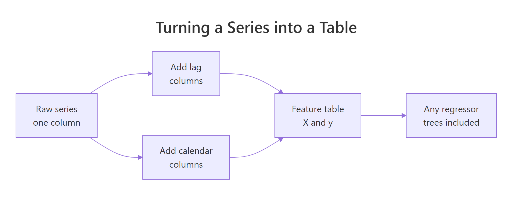
Figure 1: A forecasting model reads rows, not a timeline, so the past has to be written into each row as columns.
Try it: The block below builds a 3-month lag. Change it into a 6-month lag, the value from six months earlier, and check that row 7 then holds the value from row 1.
Click to reveal solution
Explanation: rep(NA, 6) pads the front so everything slides down six positions, and passengers[1:(n - 6)] drops the last six values so the column stays the same length as y. Row 7 now carries row 1's value, which is exactly what "six months ago" means.
What is gradient boosting actually doing?
Boosting is often described as "an ensemble of weak learners", which explains nothing. Here is the actual mechanic, and it is simple enough to write in six lines of R.
Start with the dumbest possible prediction: the mean of the target, for every row. Then measure how wrong you are on each row. That error is called the residual. Now fit a very small tree, not to the target, but to the residual. That tree learns where you are too low and where you are too high. Add a small fraction of its output to your prediction. Your errors shrink. Repeat a few hundred times.
Let's watch it happen on a curve simple enough to see. We will use a wiggly function that no single small tree could ever match.
Every row gets the same prediction, 1.214, because that is the average of the whole curve. The residual column shows how far off that is at each point. At the left end of the curve the true value is near 0, so we are over-predicting by about 1.2. Our starting error, measured as root mean squared error, is 0.6604.
Now the loop. Each round fits a stump, which is a tree allowed exactly one split, to the current residuals, then adds 30% of that stump's prediction to the running total.
Three lines do the work. resid recomputes how wrong we currently are. rpart(resid ~ x, ...) fits a single split to that error, so the stump is answering "where along x am I too low, and where am I too high?". Then pred + lr * predict(stump, toy) nudges the prediction in the direction the stump suggests, but only 30% of the way.
The remaining rpart arguments switch off machinery we do not want here. cp = 0 turns off the automatic pruning that would otherwise discard a split it judges too small to keep, and xval = 0 skips rpart's own internal cross validation, which we never look at.
The error falls every round, from 0.6604 to 0.3091, and it has more than halved after five rounds. No individual stump is any good. A single split cannot describe a sine wave. But a few hundred of them, each cleaning up after the last, can trace almost any shape.
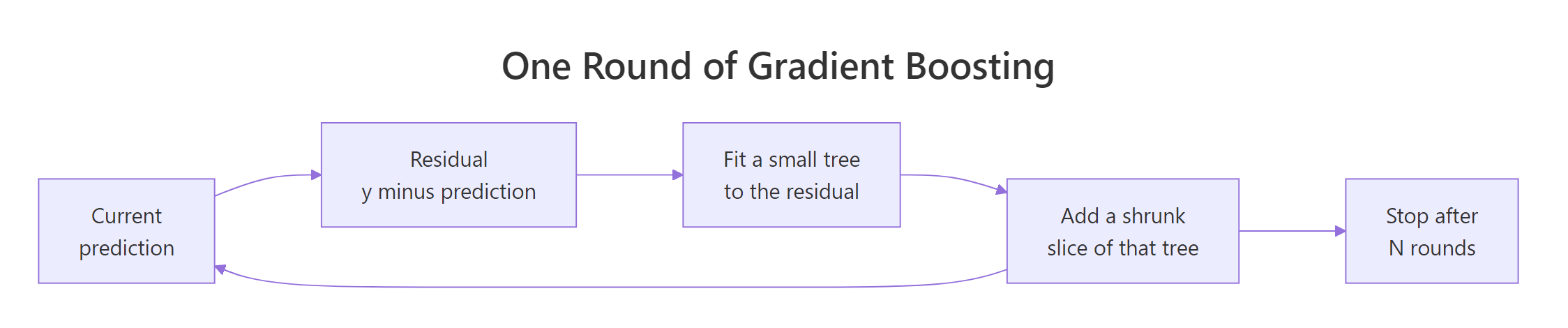
Figure 2: Each boosting round fits a small tree to what the ensemble still gets wrong, then adds a shrunk slice of it.
That lr value has a name: the learning rate, written as eta in xgboost. It is the single most important dial in boosting. Small values mean each tree contributes little, so you need more of them, but the ensemble is less likely to chase noise.
If you want the formal version, here it is. Otherwise skip to the next section, because the loop above is the whole idea.
The model after $m$ rounds is just the previous model plus a shrunken new tree:
$$F_m(x) = F_{m-1}(x) + \nu \, h_m(x)$$
Where:
- $F_m(x)$ = the ensemble's prediction after $m$ rounds
- $\nu$ = the learning rate, the fraction of each tree you keep
- $h_m(x)$ = the tree fitted at round $m$
And that tree is fitted to the residuals from the round before:
$$r_i = y_i - F_{m-1}(x_i)$$
The word "gradient" enters because when your loss is squared error, the residual is exactly the negative gradient of the loss with respect to the prediction. Fitting a tree to the residual is therefore a step of gradient descent, with one difference from the usual version: each step adds a whole function, the new tree, to the model, instead of nudging a numeric parameter. Change the loss to something else, say absolute error, and you fit each tree to that loss's gradient instead. The loop never changes.
Try it: Rerun the same five rounds with a learning rate of 0.05 instead of 0.3. Use ex_pred so you do not disturb the running example. Does the error fall faster or slower?
Click to reveal solution
Explanation: After five rounds the error has only fallen from 0.6604 to 0.5607, against 0.3091 with the larger rate. A small learning rate is not worse, it is slower on purpose. It needs many more rounds, and in exchange it usually generalises better. Learning rate and number of rounds are two ends of the same trade-off, which is why you tune them together.
How do you fit boosted trees to a real series?
Now we point that loop at the airline data. The function below is the same six lines, wrapped so we can reuse it. It adds two things: a list of feature names, and a running prediction for a held-out test set alongside the training one.
Three details matter. The fml line is only string assembly: paste glues the feature names together into the text .resid ~ lag12 + lag24 + month + t, and as.formula turns that text into a formula rpart will accept. Each round then writes the current residual into a column called .resid and fits the tree to that, which is the same trick as before. And the same tree is applied to both the training rows and the test rows, so the test predictions are built up from trees that never saw a single test row.
The split is deliberate. Everything up to December 1959 trains the model, and all of 1960 is held out. We never shuffle, because a forecast is a statement about the future and the test set has to sit in the future.
lag12 is January 1959, which is real observed history at forecast time, so no prediction is being fed back into another prediction. That keeps this comparison clean against a 12-month ARIMA forecast later on. When your features need values you will not have yet, you need recursive or direct multi-step forecasting, both covered in the feature engineering tutorial.Let's forecast 1960.
January is nearly perfect: 419.1 against an actual 417. February, June and November are all close. The model has clearly learned the seasonal shape, because it knows that month 7 should be high and month 11 should be low.
But look at July and August. Actual 622, forecast 545.3. Actual 606, forecast 548.9. Those two months are wrong by 77 and 57 passengers, and they are wrong in the same direction. That is not noise. Let's put a number on it.
Three ways of measuring the same twelve misses. Mean absolute error says the typical miss is about 25 passengers. Root mean squared error is 34.66, and the fact that it is meaningfully larger than the MAE tells you a few big misses are doing the damage, because squaring punishes large errors hardest. Mean absolute percentage error puts the typical miss at 4.92% of the true value.
An average miss of 5% sounds respectable. Hold that thought.
Try it: The block below finds the month the model most badly over-forecast. Change the last line so it finds the largest miss in either direction instead.
Click to reveal solution
Explanation: Wrapping the error in abs() changes the answer from March to July. The starter reported month 3, a 55-passenger over-forecast, but the real worst miss is month 7, under-forecast by 76.7 passengers, with August close behind at 57.1. Those are the two highest months of the year. The model is not randomly wrong, it is specifically wrong at the top of the range, and the next section explains exactly why. The output prints two numbers because the error vector kept its row names: 139 is the row label and 7 is the position we want.
Why does the forecast flat-line when the series is trending?
The July and August misses were not bad luck. They are a hard structural limit, and three numbers make it undeniable.
The busiest month in the training data had 559 passengers. The highest number this model will produce for any input whatsoever is 548.9. And July 1960 actually saw 622.
The model did not merely fail to predict 622. It cannot predict 622. There is no combination of feature values you could hand it that would produce a number above roughly 549. The forecast is pressed against a ceiling that the training data set for it.
Here is the reason, stripped to its bones. Every prediction a tree makes is a leaf average, exactly as described at the top of this page, and an average of a set of numbers can never exceed the largest number in that set. Boosting adds many trees together, so the ceiling is not exactly the training maximum, but it is always bounded by what the training targets contained. Nothing in the mechanism can produce a value above the range it was trained on.
Watch it happen on data so simple there is nowhere to hide. We fit a tree to a perfectly straight line, y equals t, for t from 1 to 20, then ask it about the future.
Inside the training range the tree is perfect: t equals 18 gives 18, t equals 20 gives 20. Step one place beyond and it returns 20. Ask about t equals 100, and t equals 1000, and it still says 20. The relationship could not be more obviously linear, and the tree still does not extend it, because "keep going up" is not a thing a tree can represent. Every prediction it can make is a leaf average from data it has already seen.
This is the single most important thing to understand about tree-based forecasting. It is why a method that dominates tabular machine learning can quietly produce a hopeless forecast the moment your series trends upward.
Try it: The block below asks the tree about three points inside its training range, where it does fine. Change them to 50, 500 and 5000 to push it far into the future, and compare what comes back with the largest value it was ever trained on.
Click to reveal solution
Explanation: Inside the training range the starter block was perfect, returning 5, 10 and 15 exactly. Step outside and all three predictions collapse to 20, the largest value in the training target. Multiplying the input by 100 changes nothing, because once a row falls into the right-most leaf, there is no right-er leaf to fall into. The prediction saturates and stays there forever.
How do you fix the trend problem?
The instinct is to reach for a bigger model: more rounds, deeper trees, more features. That does not work, and you will prove it to yourself in the practice exercises. The ceiling is a property of what trees are, not of how big they are.
The fix is to change what you ask the model to predict. Instead of predicting the passenger count, predict how much the count changed compared to the same month last year. Growth stays in a stable, familiar range even while the level keeps climbing, so the ceiling stops being a problem.
January 1951 had 145 passengers against 115 a year earlier, so growth is 30. These growth numbers sit in the tens while the levels sit in the hundreds, and crucially they do not systematically escape their historical range the way the levels do.
Now we predict growth and add last year's actual value back on to recover a passenger count. Note that lag12 drops out of the feature list, because it is now baked into the target itself.
Look at July. The level model said 545.3 against an actual 622. The growth model says 602.7. August goes from 548.9 to 616.0 against an actual 606. The ceiling is gone, because the model is no longer being asked to produce a number it has never seen. It produces a growth figure, and test$lag12 supplies the level.
Overall the error nearly halves, from RMSE 34.66 to 17.98. The model is unchanged: same trees, same rounds, same learning rate. Only the question changed.
Run that block and the shape of the problem becomes obvious. All three lines track each other closely through the first half of the year. Then the actual line spikes into the summer peak, the growth line follows it up, and the levels line flattens out exactly where the ceiling stops it.
Differencing against the same month last year is not the only option. A first difference, the change from the previous month, works when the seasonal pattern is weak. A ratio works when the series grows multiplicatively. A third route is to fit a linear trend first and boost the residuals, which is the hybrid we come back to at the end.
Try it: Try a ratio target instead of a difference. The block below builds the ratio correctly but then rebuilds the forecast with the wrong operator. Fix the reconstruction so it undoes a division rather than a subtraction.
Click to reveal solution
Explanation: Multiplying instead of adding takes RMSE from the starter's 49.63 down to 20.27. That gap is the whole lesson about target transforms: whatever you do to the target, you must exactly undo when you rebuild the forecast, and a mismatched inverse produces numbers that look plausible while being worse than doing nothing. Once the inverse is right, the ratio target beats the levels model's 34.66 and lands just behind the difference target's 17.98. The gap between ratio and difference is small enough on one test window that you should not read much into it. Both work because both keep the target range-stable, which was the actual problem.
How do you run this with the real xgboost package?
Everything so far ran on a hand-written loop, which was the point: you have now seen the entire mechanism. Production code uses xgboost, which is the same algorithm with second-order gradients, regularisation, clever split-finding and heavily optimised C++ behind it.
xgboost package is compiled C++ and needs a local R installation, so unlike every other block on this page you cannot press Run on these. Install it once with install.packages("xgboost") and paste them into RStudio. The outputs shown were captured from a real run on R 4.6.0 with xgboost 3.2.1.1.xgboost does not take a data frame and a formula. It takes a numeric matrix wrapped in its own container, xgb.DMatrix, which holds the features and the label together in a memory-efficient layout.
library(xgboost)
packageVersion("xgboost")
#> [1] '3.2.1.1'

dtrain <- xgb.DMatrix(data = as.matrix(train[, feats]), label = train$y)
dtest  <- xgb.DMatrix(data = as.matrix(test[, feats]))
dtrain
#> xgb.DMatrix  dim: 108 x 4  info: label  colnames: yes
as.matrix is doing real work here. xgboost accepts only numeric matrices, so factors and characters must be converted to numbers or one-hot encoded before this point. Our month column is already numeric, which is why we built it that way.
Now fit the same model we fit by hand, on raw levels, so you can confirm the ceiling was never an artefact of my simplified loop.
set.seed(11)
fit_level_xgb <- xgb.train(
  params = list(objective = "reg:squarederror", eta = 0.1, max_depth = 3,
                subsample = 0.9, colsample_bytree = 0.9),
  data = dtrain, nrounds = 200, verbose = 0
)
xgb_level <- predict(fit_level_xgb, dtest)

cat("highest value it ever predicts:", round(max(xgb_level), 1), "\n")
#> highest value it ever predicts: 557.6
cat("highest value it ever saw:     ", max(train$y), "\n")
#> highest value it ever saw:      559
cat("RMSE:", round(rmse(test$y, xgb_level), 2), "\n")
#> RMSE: 30.92
There it is again. The most this model will ever output is 557.6, against a training maximum of 559 and a July 1960 actual of 622. A production-grade implementation with regularisation and second-order optimisation hits precisely the same wall, because the wall is built into what a decision tree is.
The parameters map one-to-one onto the loop you already understand.
| xgboost parameter | Our loop | What it controls |
|---|---|---|
eta |
lr |
Fraction of each tree that gets added |
nrounds |
rounds |
How many trees to fit |
max_depth |
depth |
How many splits deep each tree goes |
subsample |
not used | Fraction of rows sampled per tree |
colsample_bytree |
not used | Fraction of features sampled per tree |
objective |
fixed to squared error | Which loss to take gradients of |
Now the growth target, in xgboost.
gfeats   <- c("lag24", "month", "t")
dtrain_g <- xgb.DMatrix(data = as.matrix(train[, gfeats]), label = train$growth)
dtest_g  <- xgb.DMatrix(data = as.matrix(test[, gfeats]))

set.seed(11)
fit_growth_xgb <- xgb.train(
  params = list(objective = "reg:squarederror", eta = 0.1, max_depth = 3,
                subsample = 0.9, colsample_bytree = 0.9),
  data = dtrain_g, nrounds = 200, verbose = 0
)
xgb_growth <- test$lag12 + predict(fit_growth_xgb, dtest_g)

cat("RMSE:", round(rmse(test$y, xgb_growth), 2),
    " MAPE:", round(mape(test$y, xgb_growth), 2), "%\n")
#> RMSE: 19.99  MAPE: 3.26 %
RMSE falls from 30.92 to 19.99, the same roughly-one-third improvement the hand-written loop produced. The conclusion holds across implementations: the target transform, not the library, is what rescued this forecast.
xgboost can also tell you which features it leaned on.
xgb.importance(model = fit_growth_xgb)
#>    Feature       Gain     Cover Frequency
#>     <char>      <num>     <num>     <num>
#> 1:       t 0.67187521 0.5304629 0.4176471
#> 2:   lag24 0.23536180 0.3613106 0.3991597
#> 3:   month 0.09276298 0.1082265 0.1831933
Gain is the share of error reduction each feature delivered across all splits, so it is the column to read. The time index t accounts for 67% of it, which makes sense: growth itself accelerates over these twelve years, and t is how the model tracks that. lag24 contributes 24%, and month only 9%, because much of the seasonal pattern has already been removed by differencing against the same month last year.
Finally, the honest way to choose nrounds. You hold out a slice of history, watch the error on it each round, and stop when it stops improving. The validation slice must come after the training slice in time.
fit_rows <- d[d$t <= 96, ]                    # through 1956
val_rows <- d[d$t > 96 & d$t <= 132, ]        # 1957 to 1959
fit_rows$growth <- fit_rows$y - fit_rows$lag12
val_rows$growth <- val_rows$y - val_rows$lag12

dfit <- xgb.DMatrix(as.matrix(fit_rows[, gfeats]), label = fit_rows$growth)
dval <- xgb.DMatrix(as.matrix(val_rows[, gfeats]), label = val_rows$growth)

set.seed(11)
fit_es <- xgb.train(
  params = list(objective = "reg:squarederror", eta = 0.05, max_depth = 3,
                subsample = 0.9, colsample_bytree = 0.9),
  data = dfit, nrounds = 500,
  evals = list(train = dfit, valid = dval),
  early_stopping_rounds = 30, verbose = 0
)

head(attr(fit_es, "evaluation_log"), 8)
#>     iter train_rmse valid_rmse
#>    <num>      <num>      <num>
#> 1:     1   14.67981   19.14024
#> 2:     2   14.20865   19.13839
#> 3:     3   13.90640   19.10451
#> 4:     4   13.45302   19.10672
#> 5:     5   13.03835   19.10635
#> 6:     6   12.60789   19.10255
#> 7:     7   12.20462   19.10229
#> 8:     8   11.88264   19.10231
Read the two columns against each other. Training error falls steadily, from 14.68 to 11.88 in eight rounds, and it will keep falling if you let it. Validation error barely moves, from 19.140 to 19.102, and then starts creeping back up. Of the 500 rounds we asked for, it ran 37 and picked round 7 as the best.
That gap between a training error that keeps improving and a validation error that does not is textbook overfitting, and here it starts almost immediately. The reason is the honest one: we have 72 usable training rows. Gradient boosting is a high-variance method, meaning the model it fits swings a lot when the training rows change even slightly, and it is built for tens of thousands of rows. A single monthly series with twelve years of history simply does not have enough signal to feed it. Keep that in mind for the scoreboard coming up.
Try it: Translate our hand-written call boost_trees("growth", gfeats, train, test, rounds = 400, lr = 0.02, depth = 4) into xgboost. The block below still carries the old settings, so change all three to match, then compare the score.
# Change eta to 0.02, max_depth to 4, and nrounds to 400.
set.seed(11)
ex_fit <- xgb.train(
  params = list(objective = "reg:squarederror", eta = 0.1, max_depth = 3),
  data = dtrain_g, nrounds = 200, verbose = 0
)
ex_pred_x <- test$lag12 + predict(ex_fit, dtest_g)
cat("RMSE:", round(rmse(test$y, ex_pred_x), 2), "\n")
#> RMSE: 22.23
Click to reveal solution
set.seed(11)
ex_fit <- xgb.train(
  params = list(objective = "reg:squarederror",
                eta       = 0.02,   # was lr
                max_depth = 4),     # was depth
  data = dtrain_g, nrounds = 400,   # was rounds
  verbose = 0
)
ex_pred_x <- test$lag12 + predict(ex_fit, dtest_g)
cat("RMSE:", round(rmse(test$y, ex_pred_x), 2), "\n")
#> RMSE: 20.41
Explanation: lr becomes eta, depth becomes max_depth, and rounds becomes nrounds, which sits outside the params list because it controls the training loop rather than the trees. Our loop has no equivalent of subsample or colsample_bytree, since it always uses every row and every feature. The slower, deeper settings score 20.41 against the starter's 22.23, which is a reminder that a fifth of the learning rate spread over twice the rounds is usually the safer trade.
How do you validate a forecast without fooling yourself?
Here is where a lot of published tutorials go wrong, including one of the top-ranking R articles on this exact topic. Standard machine learning practice says to use k-fold cross validation: shuffle the rows, split into five groups, train on four and test on the fifth, repeat. Applied to a time series, that procedure produces a number that is not a forecast error at all.
Let's run it anyway, on the level model, and see what it claims.
RMSE 14.85, and reassuringly consistent across the folds. If you reported that number you would be claiming this model is more than twice as accurate as the 34.66 we actually measured on 1960.
The reason is that random folds destroy the thing you are trying to measure. When you hold out a random fifth of the months, the training set still contains months from before and after each held-out month. The model is filling in gaps in the middle of history, surrounded by data on both sides. That is interpolation, and trees are excellent at it. Forecasting is extrapolation off the end, which is the one thing trees are bad at. The random split quietly replaces the hard problem with an easy one.
The correct procedure is rolling-origin evaluation. Pick a cutoff, train only on data before it, forecast the window after it, then slide the cutoff forward and repeat. Every test point stays strictly in the future of its own training set.
Five cutoffs, each followed by a 12-month forecast. The mean is 40.32, which is 2.7 times the number random folds reported. It also lands in the same neighbourhood as the 34.66 we measured on the true 1960 holdout. That agreement is the point: a trustworthy validation scheme should predict roughly what you go on to see.
Notice also that the errors are not stable across origins, ranging from 31.95 to 56.66. A single train-test split would have told you one of those numbers and hidden the other four.
Now the same harness on the growth model, which is the real test of whether the target transform was a fluke of one window.
23.92 against 40.32. The growth target wins at four of the five origins and improves the average by 41%, so the 1960 result was not a lucky window. This is the kind of evidence that should move your opinion, and a single holdout could never have provided it.
Try it: The harness below evaluates the level model at three origins with a 12-month horizon. Shorten the horizon to 6 months and see how much the numbers move.
Click to reveal solution
Explanation: The three origins give 34.68, 69.44 and 15.76, a spread of more than four to one, against 40.11, 56.66 and 39.24 at the 12-month horizon. The mean improves from 45.33 to 39.96, which is the expected direction: a shorter horizon is an easier forecast. But notice that the middle origin got substantially worse, from 56.66 to 69.44, because a 6-month window ending in mid-1958 is dominated by the fast-growing summer months where the ceiling costs the most, while the 12-month window dilutes them with easier winter months. Horizon length changes not just how hard the problem is but which part of the year you are graded on.
Does gradient boosting actually beat ARIMA and ETS, and when should you use each?
Time to answer the question in the title. We hold the split fixed, train on everything through 1959, forecast all of 1960, and score four alternatives beside our two boosted models.
The forecast package gives us all three classical benchmarks. Seasonal naive simply repeats last year's value for each month, which sounds trivial but is a genuinely hard baseline on seasonal data. ETS and auto.arima both search a family of models and keep the one with the best information criterion, a score that rewards fit and penalises extra parameters.
Both automatic searches landed on sensible models. ETS chose multiplicative errors and multiplicative seasonality with a damped additive trend, which is right for a series whose seasonal swings grow with its level. auto.arima chose one non-seasonal difference and one seasonal difference. That seasonal difference is the same year-over-year subtraction we invented by hand for the growth target, arrived at independently by a completely different tradition.
Now the scoreboard.
Read that table carefully, because it contains two lessons and only one of them is flattering to machine learning.
Boosted trees on raw levels lose to both classical models. RMSE 34.66 against 23.93 for auto.arima and 27.40 for ETS. A modern ensemble method, correctly implemented, is beaten by a technique from the 1970s, because ARIMA differences the series as a matter of routine and our level model was stuck under its ceiling.
Boosted trees on the growth target win, clearly. RMSE 17.98 against 23.93, a 25% improvement over the best classical model, and MAPE of 3.02% against 4.18%. The winning ingredient was one line of feature preparation, not the algorithm.
And seasonal naive, at RMSE 50.71, sets the floor. Any model that cannot beat it has earned nothing.
One honest caveat, because the table above is a sample of one. This is a single series and a single 12-month window. The rolling-origin test in the previous section supports the growth-target conclusion across five windows, which is much stronger evidence, but it is still one series. Do not conclude from this page that boosting beats ARIMA in general.
The wider evidence is worth knowing. In the M4 competition (2018), across 100,000 series, pure machine learning methods largely underperformed statistical ones, and the winner was a hybrid of exponential smoothing and a neural network. In the M5 competition (2020), on 42,840 related retail series with prices, promotions and calendar effects, gradient boosting dominated the leaderboard. The difference is not the algorithm's quality, it is the setting. Many related series with rich external drivers is where boosting earns its keep. A single seasonal series is where the classics are hard to beat.
Try it: Simple forecast combinations are famously hard to beat. Average the auto.arima forecast and the growth-model forecast, then score the result.
Click to reveal solution
Explanation: Combining with ARIMA scores 20.19, against 27.38 when the seasonal naive was in the mix. Averaging pulls you toward the middle of your inputs, so a weak ingredient drags the blend down and a strong one lifts it. Even the good combination at 20.19 sits behind the growth model alone at 17.98, though it comfortably beats auto.arima alone at 23.93. Combining is a large win when you cannot tell in advance which model is better, and a small loss when you can. Given how much the rolling-origin errors bounced around, "you cannot tell in advance" is the more common situation.
So when should you choose which?
The scoreboard gives you a decision rule that is more useful than "machine learning is better".
| Your situation | Reach for | Why |
|---|---|---|
| One series, a few hundred observations | ETS or ARIMA | Trend and seasonality handled natively, nothing to hand-engineer |
| Thousands of related series | Gradient boosting | One global model learns across all of them at once |
| Price, weather, promotions, holidays drive the outcome | Gradient boosting | Absorbs many external features and their interactions |
| You need prediction intervals you can defend | ETS or ARIMA | Intervals come from the model; boosting needs quantile objectives or bootstrapping |
| You must explain the forecast to a regulator | ETS or ARIMA | Parameters have meanings; a 200-tree ensemble does not |
| Sharp non-linear effects and threshold behaviour | Gradient boosting | Splits capture "above 30 degrees, demand doubles" naturally |
| Short history, long horizon | ETS or ARIMA | The extrapolation ceiling gets worse the further out you forecast |
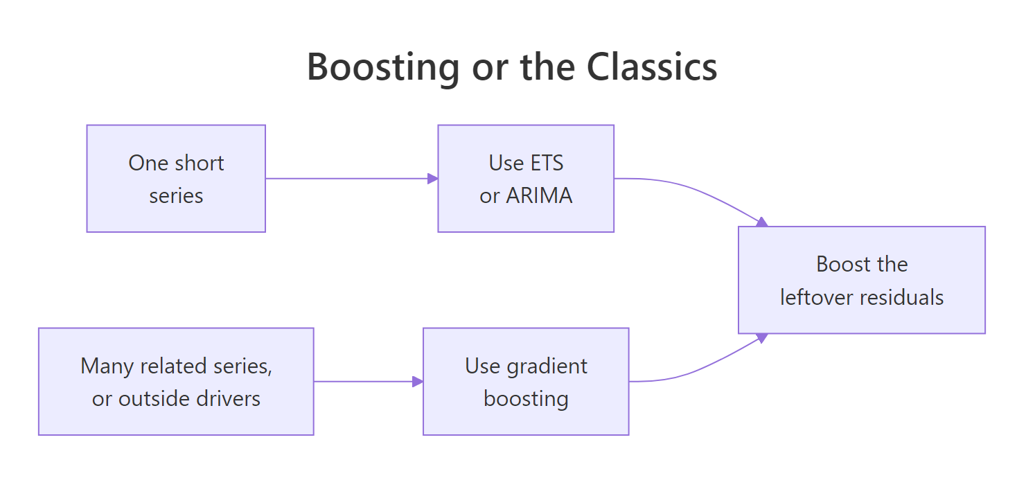
Figure 3: Series count and outside drivers decide the method, and the two families combine rather than compete.
The framing that serves you best in practice is not either-or. Let a classical model handle what it is built for, trend and seasonality, then let boosting model whatever is left over. Fit auto.arima, extract the residuals, and boost those against your external features. The M4 winner was a hybrid of exactly this spirit, and our growth target was already a half-step in the same direction: we borrowed ARIMA's seasonal differencing and handed the remainder to the trees.
Try it: Apply the first row of that table to our own data. How many rows did our feature table actually give the model, and what does the rule say we should have used?
Click to reveal solution
Explanation: The raw series has 144 months, but only 120 rows survive the lag features and only 108 of those were available for training. That is one series with a few hundred observations at most, so the table says ETS or ARIMA. And that is honestly the right call here: our growth model did win, but it took a trend diagnosis, a target transform and a rolling-origin study to get there, while auto.arima needed one line and no supervision. The early-stopping run made the same point from the other side, halting after 7 useful rounds because there was not enough data to support more.
Complete Example: an end-to-end forecast in one block
Everything above, compressed into a single self-contained script. It rebuilds the feature table, splits on time, trains the growth model, and scores it against auto.arima on the same twelve months.
Month by month the two forecasts are closer than the RMSE gap suggests. ARIMA is better in August and December, the boosted model is better in most other months, and both nail the summer peak that defeated the level model. The boosted model's edge comes mainly from March and November, where ARIMA overshoots by roughly 50 and 37 passengers respectively.
Practice Exercises
These combine several ideas from the page. Every one uses variable names starting with my_ so nothing you write here overwrites the tutorial's state.
Exercise 1: Does the growth target still help over a longer horizon?
Rebuild the split so training stops at t equal to 120, the end of 1958, and the test set covers the full 24 months of 1959 and 1960. Fit both the level model and the growth model, and report RMSE and MAPE for each. Also print the training maximum next to the level model's highest forecast.
Click to reveal solution
Explanation: Both models get worse over 24 months, which is expected since the horizon doubled and the training set shrank. The growth target still helps substantially, cutting RMSE from 50.78 to 34.81. And the ceiling is visible again: the training maximum is 505, the level model's highest forecast is 493.8, and 1960 reaches 622. The further out you forecast a growing series, the more damage that ceiling does.
Exercise 2: Can more model capacity break the ceiling?
The natural reaction to an under-forecast is to make the model bigger. Test that directly. Refit the level model on the original split with 1000 rounds and depth 6 instead of 200 and depth 3, then compare its highest forecast against the plain version and against the training maximum. Report the RMSE too.
Click to reveal solution
Explanation: Five times the rounds and twice the depth moved the ceiling from 548.9 to 558.8, and it is still below the training maximum of 559, still nowhere near July's 622. RMSE improved from 34.66 to 34.25, which is nothing. Extra capacity lets the ensemble press harder against the ceiling but can never lift it, because the ceiling comes from leaf averages, not from model size. This is the experiment that proves the fix has to be a target transform.
Exercise 3: Build a fair head-to-head harness
Score the growth model and auto.arima against each other properly, over three origins at t equal to 96, 108 and 120, with a 12-month horizon each. At every origin, retrain both models on that origin's history only, then forecast the next twelve months. Return a data frame with one row per origin and print the two means.
Click to reveal solution
Explanation: Averaged over three origins the two methods are effectively tied, 27.77 against 28.28, and they win at different origins: boosting at 96 and 120, ARIMA at 108. That is a far more honest picture than the single 1960 window, where boosting looked like a decisive 25% winner. It is also the strongest argument on this page for evaluating over multiple origins before you believe any comparison, including the one in this tutorial.
Frequently Asked Questions
Does gradient boosting require a stationary series? Not formally, since there is no statistical assumption to violate. Practically, yes: a trending target puts you under the extrapolation ceiling, so you difference or detrend for the same reason ARIMA does, arriving there by engineering rather than by theory.
Should I forecast multiple steps recursively or train a separate model per horizon? Recursive forecasting feeds each prediction back as the next step's lag, which is compact but lets errors compound. Direct forecasting trains one model per horizon, which avoids compounding at the cost of many models. This page sidestepped the choice by using only lags of 12 months and more, so every test row's features were observed history. Both strategies are worked through in the feature engineering tutorial.
How much data do I need before boosting is worth it? There is no threshold, but the early-stopping run here is instructive: with 72 training rows it found only 7 useful rounds. As a rough guide, a few thousand rows makes boosting competitive, and its real advantage appears when you can pool many related series into one global model. Below a few hundred rows, prefer the classical methods.
Can I get prediction intervals from a boosted forecast? Not directly. ARIMA and ETS derive intervals from their error model; boosting has no equivalent. The practical routes are training separate models with a quantile objective (reg:quantileerror in current xgboost) to get upper and lower bounds, or bootstrapping the residuals from a rolling-origin evaluation. Both are more work than the one-line interval you get from forecast().
Is xgboost the right choice, or should I use lightgbm or ranger? For forecasting, LightGBM is usually faster on wide feature tables and won M5, while xgboost is more widely documented and installed. ranger fits random forests rather than boosted trees, so it hits the same extrapolation ceiling and needs the same target transform. The ceiling and the validation rules on this page apply identically to all three, because they are all tree ensembles.
Summary
| Idea | What to remember |
|---|---|
| The reframing | Trees read rows, not timelines, so lags and calendar columns must carry the past into each row |
| The boosting loop | Start at the mean, fit each new tree to the current residual, add a shrunken slice, repeat |
| Learning rate | Smaller rate needs more rounds; tune the pair together, or let early stopping choose the rounds |
| The extrapolation ceiling | A tree ensemble can never predict beyond the range of its training target: 548.9 was the ceiling against a real 622 |
| More capacity does not help | 1000 rounds at depth 6 moved the ceiling to 558.8, still under the training maximum of 559 |
| The fix | Change the target, not the model: a growth target cut RMSE from 34.66 to 17.98 |
| Validation | Random 5-fold claimed 14.85, rolling origin measured 40.32; only the second is a forecast error |
| The scoreboard | Levels lost to auto.arima (34.66 vs 23.93); growth beat it (17.98); seasonal naive floor was 50.71 |
| Choosing a method | One short series favours ETS and ARIMA; many series with external drivers favour boosting |
| The hybrid | Let a classical model take trend and season, and boost whatever residual is left |
References
- Chen, T. and Guestrin, C. XGBoost: A Scalable Tree Boosting System. KDD 2016. Link
- xgboost R package documentation, including
xgb.trainandxgb.DMatrix. Link - Friedman, J. H. Greedy Function Approximation: A Gradient Boosting Machine. Annals of Statistics 29(5), 2001. Link
- Hyndman, R. J. and Athanasopoulos, G. Forecasting: Principles and Practice, 3rd edition, Chapter 5.10 on time series cross validation. Link
- Hyndman, R. J. and Athanasopoulos, G. Forecasting: Principles and Practice, 3rd edition, Chapter 12.3 on prediction with machine learning methods. Link
- M Open Forecasting Center. M4-methods: code and results for the M4 competition, 100,000 series and 61 methods. Link
- M Open Forecasting Center. M5-methods: code of the winning methods and the accuracy rankings for the M5 retail competition. Link
- Therneau, T. and Atkinson, E. An Introduction to Recursive Partitioning Using the rpart Routines. CRAN vignette. Link
- Hyndman, R. J. et al. forecast: Forecasting Functions for Time Series and Linear Models. CRAN. Link
Continue Learning
- Feature Engineering for Time Series Forecasting in R builds the full lag, rolling, calendar and Fourier feature families, shows what a leak looks like, and covers recursive versus direct multi-step forecasting in depth.
- Time Series Cross-Validation in R takes rolling-origin evaluation further, including expanding versus sliding windows and how to choose the number of origins.
- ETS vs ARIMA in R compares the two classical families this page benchmarked against, so you know which one to put up as the model to beat.