Forecast Scoring Rules in R: CRPS and Pinball Loss
A forecast scoring rule is a formula that grades a whole probability distribution against the single value that actually happened, and returns one number. CRPS and pinball loss are the two that matter in practice, and both are strictly proper, which means the only way to score well on average is to report what you honestly believe. This tutorial builds both from scratch in a few lines of base R, then uses them to pick between real forecasting models.
Why does RMSE fail to grade a probabilistic forecast?
Two forecasters both predict 100 units of demand for tomorrow. One is certain, quoting a range of a couple of units either side. The other admits it could easily land ten units either way.
RMSE and MAE see one number from each, so they call it a tie no matter how the day turns out. Here is what a rule that reads the whole distribution says instead.
The function below is crps_norm(). It scores a normal forecast distribution, and lower is better. Do not worry about the formula inside yet, we derive it line by line in a later section. For now just watch what it does across three different outcomes.
Reading the code: outcomes holds three things that could happen tomorrow. The absolute_error column is what MAE would see, computed from the point forecast of 100 alone. The two CRPS columns score the same point forecast wrapped in two different spreads, a standard deviation of 2 for the confident forecaster and 10 for the honest one.
Now the interpretation. Look at the absolute_error column: it is identical for both forecasters in every row, because it is computed from a number they both reported. It has no way to tell them apart.
The CRPS columns do tell them apart, and the answer changes with the outcome. When demand lands exactly on 100, confidence pays off and the confident forecaster wins, 0.47 against 2.34. When demand collapses to 88, the confident forecaster is punished hard, 10.87 against 7.48.
That single table cannot settle which forecaster is better, because one outcome is one outcome. The confident forecaster genuinely did win when the value landed on the nose. What we need is a rule where honesty wins on average, and that is exactly what the next section demonstrates.
Try it: Score a third forecaster who reports the same 100 but with a standard deviation of 5, against an actual value of 88. Where does the middle forecaster land relative to the other two?
Click to reveal solution
Explanation: crps_norm() is vectorised over sigma, so passing the whole vector scores all three at once. At an outcome of 88 the honest forecaster still wins, and the middle spread of 5 sits neatly between the two.
What makes a scoring rule proper, and why does it matter?
Here is the property that makes a scoring rule trustworthy. A rule is proper if your best expected score comes from reporting your honest belief. It is strictly proper if honesty is the only way to get that best score. Any other report, however clever, does worse on average.
This matters because a scoring rule is not just a report card, it is an incentive. If your team is measured on a rule that can be gamed by exaggerating confidence, someone eventually will, and the published forecasts will stop describing what anyone actually believes.
We can test propriety directly rather than take it on faith. Suppose the truth really is a normal distribution centred on 100 with a standard deviation of 8. We simulate 20,000 days from that truth, then ask what CRPS a forecaster would average if they reported the correct centre but lied about the spread.
Walking through it: truth is 20,000 outcomes drawn from the real distribution. For each candidate reported standard deviation, sapply() scores all 20,000 of those outcomes against a forecast of N(100, s) and averages the scores. That average is what the forecaster would earn in the long run by reporting s.
The result is the whole point of this section. The average score bottoms out at 4.528 when the reported standard deviation is 8, which is exactly the truth. Understate it to 2 and the average score jumps to 5.469. Overstate it to 20 and it climbs to 5.912.
There is no report that beats telling the truth, which is what strictly proper means in practice.
It reads even more clearly as a curve.
The dashed red line marks the true spread of 8. The score curve has its minimum sitting right on it. Report anything else and you climb one side of the valley or the other.
Now contrast that with a point measure, using exactly the same 20,000 outcomes.
The column is flat at 6.4 all the way down. Absolute error never touched s, because the reported spread does not appear anywhere in its formula. MAE does not reward a false spread, but it does not penalise one either: every report scores the same. A forecaster graded only on MAE has no incentive to get their uncertainty right at all.
Try it: Repeat the sweep, but this time make the truth N(100, 12). Check that the minimum moves to a reported spread of 12.
Click to reveal solution
Explanation: The minimum tracked the truth to 12, exactly as propriety promises. Notice the curve is also fairly flat near the bottom, so being slightly wrong about the spread costs much less than being badly wrong.
How does pinball loss score a single quantile?
Sometimes you do not need the whole distribution graded. You need one number checked, a specific quantile, because that is what the business actually uses. Stock cover at the 90th percentile. A staffing floor at the 10th percentile.
Pinball loss is the rule for exactly that job.
The idea behind it is an asymmetry. A 90th percentile forecast is a promise that the actual value will come in below it about 90% of the time. So the two kinds of mistake are not equally bad.
Sitting above the actual is the expected case and should barely cost anything. Sitting below the actual means the promise was broken, and that should hurt roughly nine times more.
Written out, the pinball loss for a quantile forecast $q$ at level $\tau$, against an actual value $y$, is:
$$\rho_\tau(y, q) = \begin{cases} \tau\,(y - q) & \text{if } y \ge q \\[4pt] (1 - \tau)(q - y) & \text{if } y < q \end{cases}$$
Where:
- $y$ = the value that actually happened
- $q$ = the quantile you forecast
- $\tau$ = the quantile level you claimed, between 0 and 1
- $\rho_\tau$ = the penalty, always zero or positive
Both branches are just the size of the miss multiplied by a weight. The whole trick is that the two weights, $\tau$ and $1 - \tau$, are different. That is four lines of R.
Reading the code: ifelse() picks the branch element by element, so the function stays vectorised. Both calls forecast a 90th percentile of 100 and both miss by exactly 4 units, once low and once high.
The two penalties are 0.4 and 3.6, a nine-to-one ratio, from an identical 4-unit miss. That is the asymmetry doing its job. Overshooting your 90th percentile is cheap, because the actual value is supposed to land below it. Undershooting it is expensive, because the actual value blew past a level you said it would rarely reach.
Sweeping the quantile forecast across a range makes the shape obvious.
Here the actual value is fixed at 100 and the forecast moves. At $\tau = 0.5$ the two arms are symmetric: being 20 low and being 20 high both cost 10. At $\tau = 0.9$ they are not: being 20 low costs 18, while being 20 high costs only 2.
Plotting it shows where the name comes from.
Each line is a V with its point at the actual value of 100 and one arm steeper than the other. At $\tau = 0.1$ the steep arm faces right, punishing forecasts that sit too high. At $\tau = 0.9$ it faces left. At $\tau = 0.5$ the V is symmetric, which connects this rule back to something familiar.
At $\tau = 0.5$ both weights are 0.5, so the loss is exactly half the absolute error. Pinball loss is therefore a generalisation of the error measure you already know: MAE is the special case where you only care about the median.
quantile_score() function in fabletools, and the fpp3 textbook, both use twice this value so that the median case equals the absolute error rather than half of it. Rankings are unaffected because every score is doubled equally, but the printed numbers differ by a factor of two.Try it: Compute the pinball loss at $\tau = 0.1$ for the same two misses, an actual of 96 and an actual of 104 against a forecast of 100. Predict which one is penalised more before you run it.
Click to reveal solution
Explanation: The penalties flipped. A 10th percentile is supposed to sit below the actual value nearly always, so landing above it is the expensive mistake this time.
How does CRPS grade the whole forecast distribution?
Pinball loss grades one quantile. CRPS grades all of them at once, which is what you want when the deliverable is the entire distribution rather than one chosen level.
The picture behind CRPS is simple once you see it. Draw the cumulative distribution function of your forecast, an S-shaped curve rising from 0 to 1. Now draw what a perfect forecaster would have said with hindsight: a step that sits flat at 0 until the actual value, then jumps straight to 1. CRPS is the area of the squared gap between those two curves.
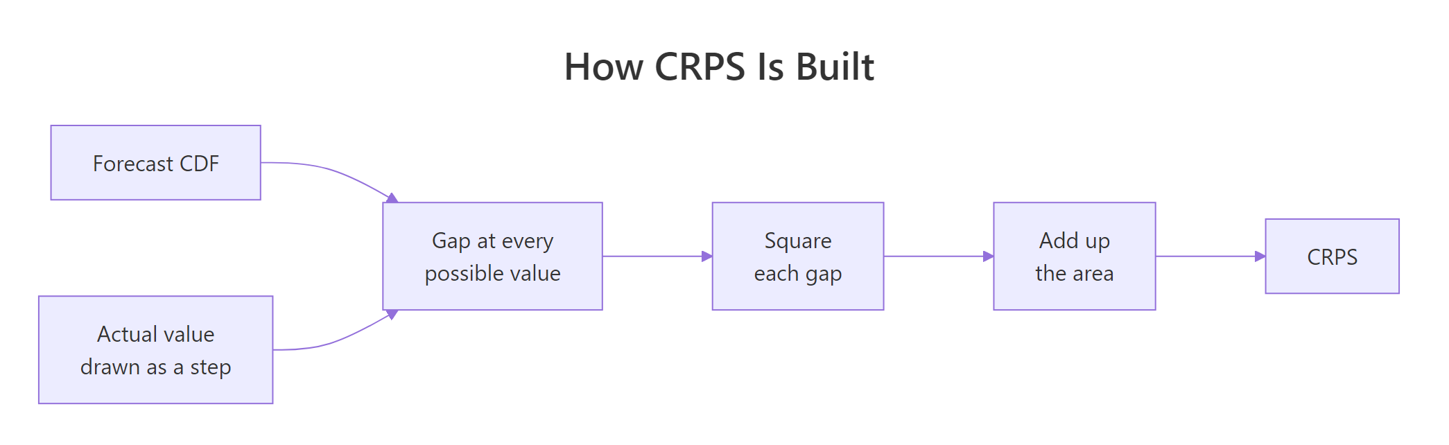
Figure 1: CRPS compares the forecast CDF with a step function at the actual value, then adds up the squared gap.
In notation, with $F$ the forecast CDF and $y$ the actual value:
$$\text{CRPS}(F, y) = \int_{-\infty}^{\infty} \big(F(u) - \mathbf{1}\{u \ge y\}\big)^2 \, du$$
Where:
- $F(u)$ = the forecast probability that the outcome is at or below $u$
- $\mathbf{1}\{u \ge y\}$ = the hindsight step, 0 below the actual value and 1 at or above it
- the square = why both being wrong and being vague are penalised
- $du$ = we sweep across every possible value $u$ and add up as we go
If the notation is not your thing, skip to the code. The integral is doing nothing more than measuring the gap in the figure above.
Because the formula is literally an area, we can compute it with R's numerical integrator and check it against the closed form we have been using all along.
Walking through it: gap_squared() is the integrand, the squared difference between the forecast CDF at u and the hindsight step at u. The comparison u >= y returns TRUE or FALSE, which R treats as 1 or 0 in arithmetic. integrate() then sweeps that function across a range wide enough to capture essentially all the probability, twelve standard deviations either side.
The two numbers agree to four decimal places. That confirms crps_norm(), the function we have been trusting since the first section, is nothing but this area computed with pen and paper instead of a numerical integrator. For a normal forecast that closed form is:
$$\text{CRPS} = \sigma\left[ z\big(2\Phi(z) - 1\big) + 2\varphi(z) - \tfrac{1}{\sqrt{\pi}} \right], \qquad z = \frac{y - \mu}{\sigma}$$
Where $\Phi$ is pnorm(), $\varphi$ is dnorm(), and $z$ is how many standard deviations the actual value sat from the forecast mean. Compare it to the R function from the first section and you will find the two match term for term.
Seeing the gap helps more than either formula.
The blue S-curve is the forecast, the red step is hindsight, and the shaded band between them is the gap. CRPS squares that gap before adding it up, so the shaded region is the thing being measured rather than the answer itself.
A sharper forecast centred on 96 would make the blue curve hug the red step and shrink the band. A vague forecast would flatten the blue curve and widen it. Both ways of being wrong grow the same area, which is precisely why the rule cannot be gamed.
Try it: Score an actual value of 96 against three forecasts that share a standard deviation of 10 but are centred on 96, 100 and 104. Confirm the centred forecast wins, and that missing high by 4 costs more than being spot on.
Click to reveal solution
Explanation: crps_norm() vectorises over mu just as it did over sigma. Being centred on the truth scores best at 2.337. Notice the penalty grows faster than the miss does: moving the centre 4 units off adds 0.63 to the score, while moving it 8 units off adds 2.43, nearly four times as much rather than twice as much.
Why is CRPS just the average of every pinball loss?
Two sections ago we scored one quantile. One section ago we scored a whole distribution. Those look like separate tools, but they are the same tool at different resolutions, and the link between them is the most useful fact in this tutorial.
A distribution is nothing more than all of its quantiles stacked together. So if you score every quantile with pinball loss and average the results, you have scored the whole distribution. That average, doubled, is exactly CRPS:
$$\text{CRPS}(F, y) = 2 \int_{0}^{1} \rho_\tau\big(y,\; F^{-1}(\tau)\big) \, d\tau$$
Where $F^{-1}(\tau)$ is the forecast's $\tau$-th quantile, which in R is qnorm(tau, mu, sigma) for a normal forecast.
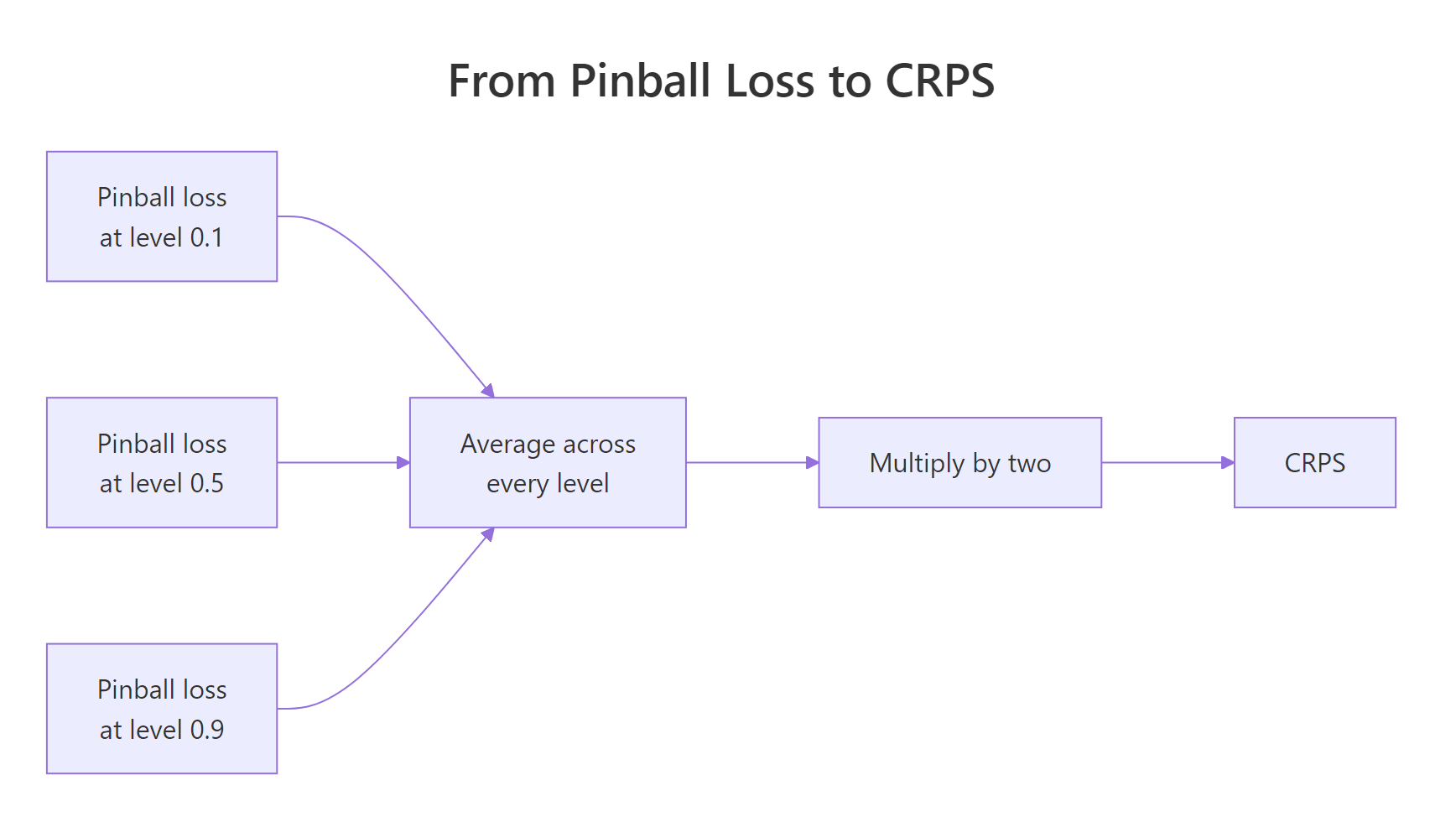
Figure 2: CRPS is the average pinball loss across every quantile level, doubled.
We can check the claim rather than believe it. Take a thousand quantile levels spread evenly between 0 and 1, score each one with the pinball() function we wrote earlier, then average.
Reading the code: tau_grid is a thousand quantile levels, deliberately stopping just short of 0 and 1 where the normal quantiles run off to infinity. q_grid converts each level into the matching quantile of the forecast distribution. Then pinball() scores the actual value of 96 against all thousand quantiles at once, and mean() averages them.
The two numbers are identical to four decimal places, and neither one knew about the other. The left number was built by scoring a thousand separate quantiles. The right number came from an integral of a squared area. They agree because they are the same quantity.
This identity has a practical payoff. Many modern forecasters, including quantile regression and gradient boosting with a quantile objective, output a set of quantiles rather than a named distribution. You can score them directly by averaging pinball losses across the quantiles they produced, with no distributional assumption at all.
Try it: Verify the identity again with different numbers. Score an actual value of 57 against a forecast of N(50, 4), both ways.
Click to reveal solution
Explanation: The identity holds for any normal forecast and any actual value. Only q_grid had to change, because the quantile levels themselves are the same thousand numbers regardless of which distribution you are scoring.
How do you score a forecast made of simulated draws?
Not every forecast has a tidy formula behind it. Bootstrapped forecasts, simulated future paths and ensemble models all hand you a bag of possible outcomes rather than a named distribution. CRPS handles that case too, with a different but equivalent formula.
For a set of draws $X_1, \dots, X_n$ from your forecast distribution:
$$\text{CRPS} = \frac{1}{n}\sum_{i} |X_i - y| \;-\; \frac{1}{2n^2}\sum_{i}\sum_{j} |X_i - X_j|$$
Where:
- the first term = how far your draws sit from what actually happened, on average
- the second term = how spread out your draws are among themselves, on average
- $y$ = the actual value
The two terms are worth pausing on because together they are the whole philosophy of the rule. The first term rewards accuracy, since draws close to the truth make it small. On its own it would reward cheating: predict the same number a thousand times with no spread at all and you would just get absolute error.
The second term stops that. It is subtracted, so a forecast that spreads its draws out gets a credit, and a forecast that collapses to a point gets no credit at all. Accuracy and honest uncertainty are traded off inside one formula.
Walking through it: outer(draws, draws, "-") builds every pairwise difference as a 1000 by 1000 matrix, and taking the mean of its absolute values gives the average distance between two random draws. The first term is the average distance from the draws to the actual value. Subtracting half the second from the first gives the score.
The interpretation is the useful part. We deliberately drew from N(100, 10), the same distribution we scored in closed form earlier, and the two routes give 2.9946 and 2.9669. The small gap is sampling error from using only 1000 draws, not a disagreement about the formula. With more draws it shrinks toward zero.
Worth confirming against a package that specialises in this. The block below uses scoringRules, which is not available in the browser, so run it locally in RStudio if you want to reproduce it.
round(c(
  ours_closed = crps_norm(96, 100, 10),
  pkg_closed  = scoringRules::crps_norm(y = 96, mean = 100, sd = 10),
  ours_draws  = crps_from_draws(96, draws),
  pkg_draws   = scoringRules::crps_sample(y = 96, dat = draws)
), 6)
#> ours_closed  pkg_closed  ours_draws   pkg_draws
#>    2.966881    2.966881    2.994630    2.994630
Both of our hand-written functions match the reference implementation to six decimal places. They are not simplified teaching versions: they compute exactly what the published package computes.
Try it: Score the same actual value of 96 using 200 draws and 2000 draws, and compare both against the closed form. Which sample size lands closer?
Click to reveal solution
Explanation: The 200-draw estimate is off by about 0.09, the 2000-draw estimate by about 0.02. Sampling error shrinks roughly with the square root of the number of draws, so ten times more draws buys you about three times the precision.
How do you score real fable forecasts with accuracy()?
Time to apply all of this to actual models. The fable package computes every rule in this tutorial through one function, accuracy(), and the numbers it returns are the ones we have been building by hand.
The data is Australian quarterly beer production from tsibbledata, measured in megalitres. We hold back everything from 2008 onwards so there are ten real quarters to grade against, and fit four models that disagree with each other in interesting ways.
Walking through it: filter_index() trims the series by time. Given two quarters either side of a ~, it keeps everything between them, which is how we cut the series down to 1992 Q1 through 2010 Q2. Given a ~ with nothing on its left, as in filter_index(~ "2007 Q4"), it keeps everything up to and including that quarter, which is how we carve off the training period. model() fits all four candidates in one call, and forecast(h = 10) produces ten quarters ahead from each.
The last three lines are only there to show what came back. A forecast object carries two things per quarter: a Beer column that is not a number at all but a <dist> column holding a whole normal distribution, and a .mean column holding the single point forecast pulled out of it. format() turns the distribution into readable text so both can sit in one printed table. That <dist> column is exactly the object our scoring rules need.
One thing to read carefully: N(426, 164) means a normal distribution with mean 426 and variance 164, so a standard deviation of about 12.8. The second number is a variance, not a standard deviation, and reading it as a standard deviation is an easy mistake to make.
Start with the point measures, which grade only the .mean column.
Note that we scored against beer, the full series, not against train. The accuracy() function finds the 2008 to 2010 actuals in there and lines them up with the forecasts by quarter.
Already the two point measures disagree with each other. RMSE ranks ets first at 9.80, while MAE ranks tslm first at 7.27 by a comfortable margin. That happens when one model has smaller typical errors but a couple of larger ones, since RMSE squares errors and so punishes the occasional big miss harder.
Now add CRPS, which reads the whole <dist> column instead of just .mean.
This is the moment the tutorial has been building toward. On MAE, tslm is the clear winner at 7.27 against 8.99 for ets, a 19% margin. On CRPS the order reverses and ets wins, 5.82 against 5.86. The two models are nearly tied once you grade the whole distribution, and the model with visibly worse point forecasts comes out ahead.
The reason is that CRPS is grading something MAE never looked at. The tslm model puts its centre in a better place, but ets describes its own uncertainty slightly better, and that is enough to close a 19% gap. If your deliverable is an interval or a risk number rather than a single point, the CRPS ranking is the one that matters.
train instead of beer to accuracy() returns training-set residual measures, which flatter complex models and are close to meaningless for choosing between them. The .type column tells you which you got: it must say Test.You can also grade one specific quantile with quantile_score(), which is the doubled pinball loss from earlier.
The probs argument names the quantile level. This is the score to report when the business only uses one number from your forecast, such as a stock cover level set at the 90th percentile. Here ets is best at 3.20 and tslm slips to third, because a model can describe the middle of a distribution well and its upper tail poorly.
Try it: Fit just ETS() and MEAN() on the same training data and compare them on CRPS. MEAN() forecasts the historical average forever, so it should lose badly on a strongly seasonal series.
Click to reveal solution
Explanation: MEAN() ignores the seasonal swing entirely, so its centre sits far from the actual value in most quarters, and the wide spread it reports to cover that error is itself penalised by the second term of the rule. A CRPS of 22.4 against 5.82 quantifies just how much the seasonal structure was worth.
How does the Winkler score grade a prediction interval?
Sometimes the thing you ship is neither a point nor a full distribution. It is an interval: "between 380 and 415 megalitres, with 80% confidence". The Winkler score is the proper rule for that deliverable.
It balances two things you would otherwise have to trade off by hand. A narrow interval is more useful, so width is a cost. But an interval that misses is a broken promise, so landing outside is a much bigger cost. Written out:
$$W_\alpha = (u - \ell) + \frac{2}{\alpha} \times \begin{cases} \ell - y & \text{if } y < \ell \\ 0 & \text{if } \ell \le y \le u \\ y - u & \text{if } y > u \end{cases}$$
Where:
- $\ell$ and $u$ = the lower and upper ends of the interval
- $\alpha$ = 1 minus the confidence level, so 0.20 for an 80% interval
- $2/\alpha$ = the penalty multiplier, which is 10 for an 80% interval and 40 for a 95% one
The multiplier is what makes the rule honest. For an 80% interval, every unit you land outside costs ten times what a unit of extra width would have cost. Shrinking an interval to look impressive is therefore a losing trade unless you are genuinely confident.
The level argument names which interval to grade. Here is the second surprise of the tutorial: tslm, which had the best MAE of any model at 7.27, now ranks third at 39.8, behind arima which had the second-worst MAE at 10.4. The best point forecaster produces the second-worst intervals.
Rather than take that on trust, we can rebuild the whole thing by hand from the intervals themselves.
Reading the code: hilo(80) extracts the 80% interval from each forecast distribution, and unpack_hilo() splits it into plain lower and upper columns. The pmax(..., 0) pair encodes the three-case formula compactly, since only one of the two can be positive at a time. The left_join() brings in the actual values.
All four numbers match accuracy() exactly. Nothing is hidden inside the package.
So where does the tslm penalty come from? Both models missed their interval in exactly one quarter out of ten, and their intervals are almost the same width. The difference is how badly they missed.
You can check the arithmetic yourself: for arima, 34.1 of width plus 35.7 of penalty gives 69.8. For tslm, 34.4 plus 54.6 gives 89.0. The widths are within 1% of each other, so essentially all of the 19-point gap comes from the penalty term.
Beer production in 2009 Q3 came in at 419, and tslm put its upper bound about 1.9 megalitres lower than arima did. You can read that straight off the penalty column: dividing 54.6 and 35.7 by the multiplier of ten gives overshoots of 5.46 and 3.57 megalitres, a difference of 1.89. Multiplying that small difference in placement back up by ten is what produced the whole 19-point gap.
That single quarter, spread over the ten-quarter average, is what moved tslm from first on MAE to third on Winkler.
Try it: Score the same four models at the 95% level instead of 80%. The penalty multiplier becomes 40, so misses matter far more. Does the ranking survive?
Click to reveal solution
Explanation: The scores rose because 95% intervals are wider and width is a cost. More interestingly, arima and ets are now tied at 51.6 where ets led clearly at the 80% level. A ranking that depends on which interval you grade is a warning that the models are genuinely close.
How do you compare scores across series of different scales?
Everything so far graded one series. The moment you forecast many series at once, a new problem appears: CRPS is measured in the units of the data, so it cannot be averaged across series that live on different scales.
Here is the problem made concrete. We put beer production, which runs in the hundreds of megalitres, alongside electricity production, which runs in the tens of thousands of gigawatt hours, into one tsibble and score both.
Walking through it: pivot_longer() stacks the two measurements into one value column with a Series label, and as_tsibble(key = Series) tells fable these are two separate series to be modelled independently. Each gets its own ETS and seasonal naive fit.
Look at the magnitudes. Electricity CRPS is around 1589, beer is around 5.82, a factor of 270. If you averaged those two numbers to get an overall model score, electricity would decide the winner on its own and beer would contribute nothing. That is not a judgement about which series matters more, it is an accident of the units.
The fix is a skill score, which converts each raw score into a percentage improvement over a benchmark model. Against a benchmark score $B$ and your score $S$:
$$\text{Skill} = \frac{B - S}{B}$$
A skill of 0.30 means you beat the benchmark by 30%. Zero means you tied it. Negative means the benchmark beat you. Because it is a ratio, the units cancel and the numbers become comparable across series.
The skill_score() wrapper takes any measure and re-expresses it against a benchmark, which by default is the seasonal naive forecast. That is why the snaive rows are exactly 0: it is being compared with itself.
Now the comparison is honest, and it delivers news that the raw table hid. On beer, ETS beats the naive benchmark by 33.2%, a solid win. On electricity it is 1.7% worse than simply repeating last year's quarter. The model that looked uniformly good is only good on one of the two series, and no amount of staring at 5.82 and 1589 would have told you that.
Try it: Average each model's skill across both series to get one overall number per model. This is the standard way to rank models over a portfolio of series.
Click to reveal solution
Explanation: Averaging 0.332 and -0.017 gives 0.157, so ETS is about 16% better than the benchmark across the portfolio. That is a defensible headline number in a way that averaging 5.82 and 1589 never could be.
Practice Exercises
Exercise 1: Build a scoring report
Produce a single report for the four beer models containing CRPS, the Winkler score at level 90, and CRPS expressed as a percentage of the mean of the beer series so it can be read as a relative error. Sort by CRPS. Save it to my_report.
Click to reveal solution
Explanation: The crps_pct column is the useful addition. A CRPS of 5.82 is meaningless without context, but 1.34% of the series mean is instantly interpretable and roughly comparable to a percentage error on another series. Note that at level 90, arima and ets tie on Winkler at 43.3 even though ets leads on CRPS, another reminder that the interval you grade changes the answer.
Exercise 2: Make RMSE and CRPS disagree
Construct two forecasters over 5,000 simulated days where the truth is N(100, 9). The first is sharp but overconfident: its centre is nearly perfect (mean plus a small wobble of sd 1) but it reports a standard deviation of only 1. The second is blunt but honest: its centre wobbles more (sd 4) but it reports the correct spread of 9. Show that the sharp model wins on RMSE while the honest model wins on CRPS.
Click to reveal solution
Explanation: The rankings are fully reversed. RMSE prefers the sharp model, 8.894 against 9.797, because its centre really is closer to the truth. CRPS prefers the honest one, 5.564 against 6.601, because the sharp model claims a spread of 1 when reality has a spread of 9, so it assigns almost no probability to what actually happens on most days. In production its actual values would fall outside its intervals constantly while its headline error looked excellent.
Exercise 3: Score a skewed forecast
A forecast of website sessions is right-skewed: 4,000 draws from a lognormal with meanlog = 3 and sdlog = 0.6. The actual value came in at 30. Score it with the draws-based CRPS, then score it again by pretending the forecast was normal with the same mean and standard deviation as the draws. How much does the normal assumption distort the answer?
Click to reveal solution
Explanation: The normal approximation reports 4.459 where the honest answer is 5.584, understating the score by about 20%. A normal distribution with the same mean and spread puts probability below zero and misses the long right tail entirely, so it flatters a forecast that is genuinely worse than it looks. When your forecast is skewed, score the draws directly and never substitute a normal with matching moments.
Frequently Asked Questions
Is a CRPS of 5.82 good? On its own, no number is good or bad, because CRPS carries the units of your data. Divide it by the series mean for a relative figure (5.82 on beer is 1.34%), or convert it to a skill score against a naive benchmark. Those two transformations are what make the number interpretable.
Why is my skill score negative? Because your model scored worse than the benchmark, which by default is the seasonal naive forecast. That is a genuinely useful finding rather than a bug, as the electricity example in this tutorial showed. A sophisticated model that cannot beat "the same quarter last year" is not earning its complexity.
Which single rule should I report? Report the rule that matches your deliverable. If you ship one number, use MAE or RMSE. If you ship one quantile, use pinball loss at that level. If you ship an interval, use the Winkler score at that level. If you ship the whole distribution or you are not sure, use CRPS, since it grades every interval at once.
Should I average CRPS across forecast horizons? Only if a one-step error and a ten-step error are equally costly to you, which is rarely true. Uncertainty grows with the horizon, so a raw average is dominated by the far end. Report scores per horizon when you can, and average only when you have a genuine reason to weight them equally.
Does a low CRPS mean my intervals are correctly calibrated? No, and this is the easiest thing to get wrong. A proper scoring rule ranks the forecasts you hand it against each other; it never certifies that any of them is good. The winner of your comparison can still be the best of a badly calibrated set, with 80% intervals that only contain the actual value half the time. Score to choose between models, then check calibration separately by counting how often the actual value fell inside your 80% interval and seeing whether that share is near 80%. Coverage is useless as a grade, since you can always widen your way to it, but it is a good diagnostic to run beside a proper score.
What about the log score? It is strictly proper and popular in Bayesian work, but it is brutal in a specific way: it returns infinity if the actual value lands where your forecast assigned zero probability. One unlucky observation can therefore destroy an otherwise good model's average. CRPS penalises the same mistake proportionately rather than infinitely, which is why it is the safer default for forecasting.
Summary
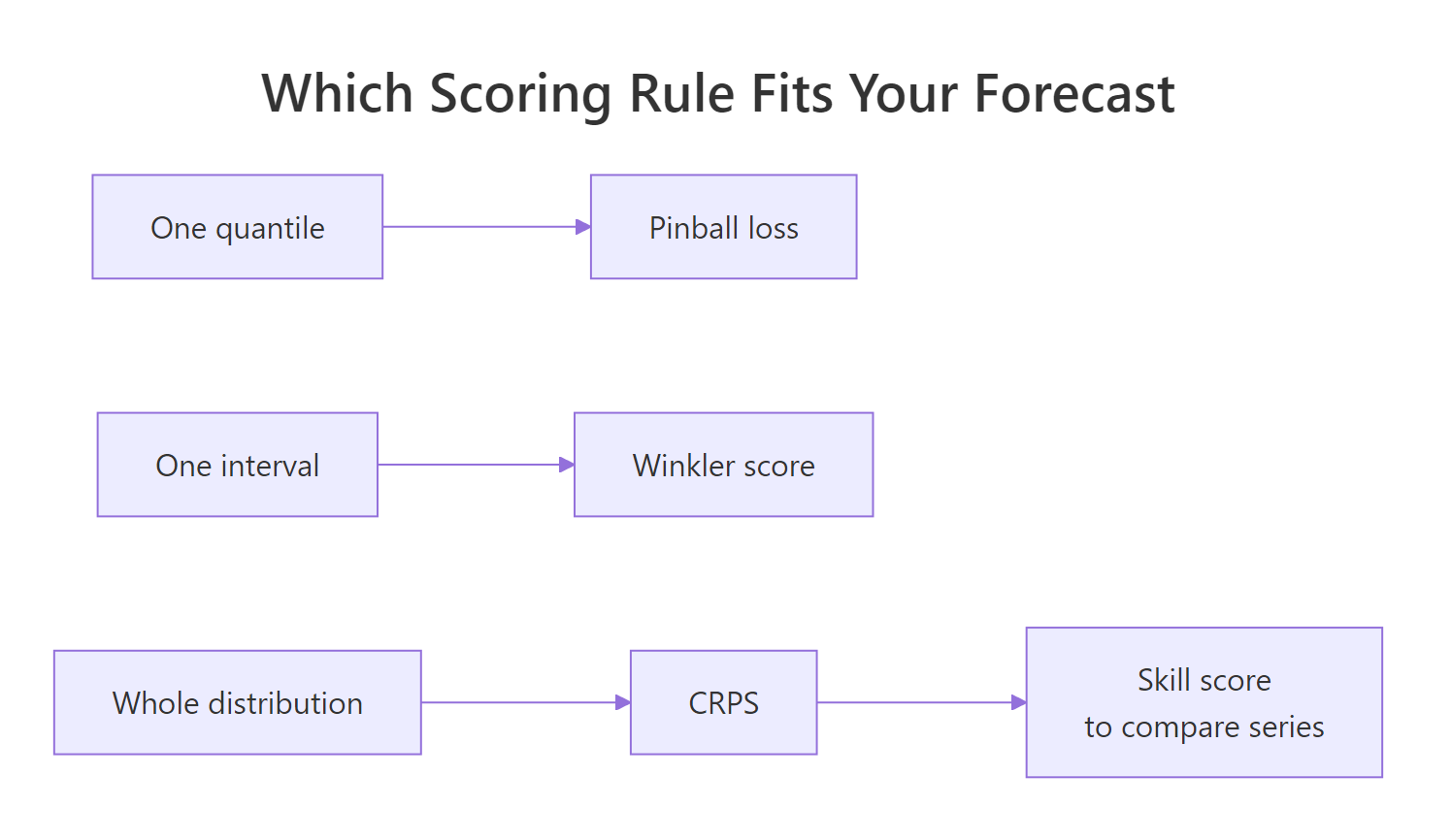
Figure 3: Match the scoring rule to what your model actually outputs.
One call scores the four beer models on every rule in this tutorial at once. This is the table you would actually put in front of a colleague.
Read it row by row and the disagreements are visible at a glance. MAE says tslm is the best model by a wide margin. CRPS says ets and tslm are effectively tied. Winkler says tslm is third. The skill column says ets beats the seasonal naive benchmark by 33%. Every one of those numbers is reproducible by hand with the functions from the first half of this tutorial, exactly as the Winkler rebuild showed.
Which row wins depends entirely on what you ship. If the deliverable is the distribution or an interval, ets is the pick. If it is a single number every quarter, tslm and its better MAE is the right call instead.
| Rule | Grades | R call | Key property |
|---|---|---|---|
| MAE / RMSE | The point forecast only | accuracy(measures = list(MAE = MAE)) |
Blind to uncertainty |
| Pinball loss | One named quantile | quantile_score with probs = |
Asymmetric penalty; MAE at the median |
| Winkler score | One named interval | winkler_score with level = |
Width plus a 2/alpha miss penalty |
| CRPS | The whole distribution | CRPS |
Average pinball across all levels |
| Skill score | Any rule, versus a benchmark | skill_score(CRPS) |
Unit-free, comparable across series |
The five things worth carrying away:
- Point measures cannot see uncertainty. RMSE and MAE read only the mean, so two models with identical means and wildly different spreads score the same.
- Proper means honesty wins on average. The 20,000-day sweep showed average CRPS bottoming out exactly at the true spread, and average absolute error staying flat regardless.
- Pinball loss and CRPS are the same rule. Score one quantile and you get pinball loss; average across all quantile levels and double it, and you get CRPS to four decimal places.
- Rankings genuinely disagree, so pick the rule that matches the deliverable. On beer production,
tslmwon on MAE,etswon on CRPS, andtslmfell to third on the Winkler score. - Never average raw scores across series of different scales. Electricity CRPS of 1589 would swamp a beer CRPS of 5.82. Convert to skill scores first.
References
- Gneiting, T. and Raftery, A. E. Strictly Proper Scoring Rules, Prediction, and Estimation. Journal of the American Statistical Association 102(477), 359-378 (2007). The foundational paper defining propriety. Link
- Hyndman, R. J. and Athanasopoulos, G. Forecasting: Principles and Practice, 3rd edition, Section 5.9: Distributional forecast accuracy. Link
- fabletools reference:
accuracy()and the distribution accuracy measures. Link - fabletools reference:
CRPS()andquantile_score(). Link - Jordan, A., Krueger, F. and Lerch, S. Evaluating Probabilistic Forecasts with scoringRules. Journal of Statistical Software 90(12) (2019). Closed forms for many distribution families. Link
- Bracher, J., Ray, E. L., Gneiting, T. and Reich, N. G. Evaluating Epidemic Forecasts in an Interval Format. PLOS Computational Biology 17(2) (2021). Formalises the interval score that Winkler introduced in 1972, and shows how it relates to CRPS. Link
- Bosse, N. I. et al. Evaluating Forecasts with scoringutils in R. arXiv:2205.07090 (2022). A survey of scoring rules and their pitfalls. Link
- Gneiting, T., Balabdaoui, F. and Raftery, A. E. Probabilistic Forecasts, Calibration and Sharpness. Journal of the Royal Statistical Society B 69(2), 243-268 (2007). The source of the sharpness-subject-to-calibration principle, and the best answer to the calibration question in the FAQ above. Link
Continue Learning
- Distributional Forecasts in R with fable shows where the
<dist>column comes from and how to pull intervals, quantiles and simulated paths out of it. Read it first if the forecast objects in this tutorial felt unfamiliar. - Forecast Accuracy in R covers the point measures in depth, including MASE and the scaled errors that solve the cross-series problem for point forecasts the way skill scores solve it here.
- Conformal Prediction in R builds prediction intervals with guaranteed coverage and no distributional assumption, which pairs naturally with the Winkler score for grading them.