Bootstrapping and Bagging Forecasts in R
Bootstrapping a time series means manufacturing many plausible alternative histories from the one history you actually observed. Bagging means fitting a forecast to each of those histories and averaging the answers. In R, bld.mbb.bootstrap() builds the alternative histories and baggedETS() turns them into a single, steadier forecast.
What does bootstrapping a time series actually do?
You only ever get one history. Every parameter your model estimates, and the model type itself, is a guess made from that single sample, and a slightly different sample would have produced slightly different guesses. Bootstrapping manufactures those "slightly different samples" so you can see how much your forecast depends on the luck of the draw. Here is what one history turned into four looks like.
AirPassengers is a built-in dataset: monthly totals of international airline passengers from 1949 to 1960. bld.mbb.bootstrap(y, n) takes that series and returns a list of n series, each the same length and each with the same overall shape.
Look at the columns side by side. January 1949 was 112 real passengers. In the three manufactured histories it is 113.3, 105.9 and 114.5. Every month wobbles a little, but the January-to-June climb is there in all four. These are not random numbers, they are answers to the question "what else could this series plausibly have looked like?"
bld.mbb.bootstrap() returns the untouched input as element one, which is why the table above starts at boot[[2]]. It is a convenience so the ensemble always contains the real data, and it catches people out when they expect all n elements to be resampled.Before going further, it helps to see the plain bootstrap on something much smaller than a time series. Suppose you measured five things and want to know how reliable their average is.
sample(x, 5, replace = TRUE) draws five values from x, putting each one back after drawing it. That is what "with replacement" means, and it is the entire trick. Here the draw picked 12 three times and never picked 11 or 18 at all.
That resample is a stand-in for "a different five measurements I could have taken." Its mean is 13, not 14. Do it a thousand times and the spread of those means tells you how much your estimate of 14 could have wobbled.
replicate(1000, ...) runs the resample-and-average step a thousand times and collects the results. quantile() then reads off the 2.5th, 50th and 97.5th percentiles of those thousand means.
The middle 95% of those means falls between 12 and 16. You never had to assume normality, never derived a standard error, never opened a textbook. Redrawing the five values you already have, a thousand times over, is enough to measure how far the answer moves. That is the bootstrap.
Try it: Repeat the same experiment for the median instead of the mean. Store the 1000 medians in ex_medians and print the 2.5%, 50% and 97.5% quantiles.
Click to reveal solution
Explanation: Only the summary function changed, from mean() to median(). The median's interval runs 11 to 18, much wider than the mean's 12 to 16, because with only five values the median jumps to whichever value lands in the middle rather than smoothing across all of them.
Why does plain resampling break a time series?
The five-number bootstrap worked because those five measurements were interchangeable. Shuffle them into any order and they still describe the same thing. A time series is the opposite: the order is the information. Here is what happens when you ignore that.
acf() measures autocorrelation: how strongly a value resembles the value that came some number of steps before it. The $acf vector starts at lag 0, so positions 2, 3 and 13 give lags 1, 2 and 12. Lag 12 matters most here because the data is monthly, so lag 12 is "the same month last year."
Read the two columns. In the real series, this month looks 0.948 like last month and 0.760 like the same month a year ago. In the shuffled copy, both numbers collapse to roughly zero. The shuffle threw away every relationship the forecasting model was going to learn from.
That is the whole problem in one table. A bootstrap of a time series has to produce something a forecasting model would still recognise as the same kind of series. Independent resampling keeps every original value and their overall distribution, but destroys the ordering that carried the information.
Try it: Do the same check on USAccDeaths, a monthly count of accidental deaths in the US from 1973 to 1978. Shuffle it into ex_shuffled and compare the lag-12 autocorrelation with the original's.
Click to reveal solution
Explanation: USAccDeaths peaks every July, so a value resembles the value 12 months earlier at 0.629. Shuffling drops that to -0.125, statistically indistinguishable from no relationship at all.
How the moving block bootstrap keeps the pattern intact
The fix is almost obvious once you see the problem. If resampling one point at a time destroys the memory between neighbours, then resample runs of consecutive points instead. Inside a run, neighbours stay neighbours and the memory survives.
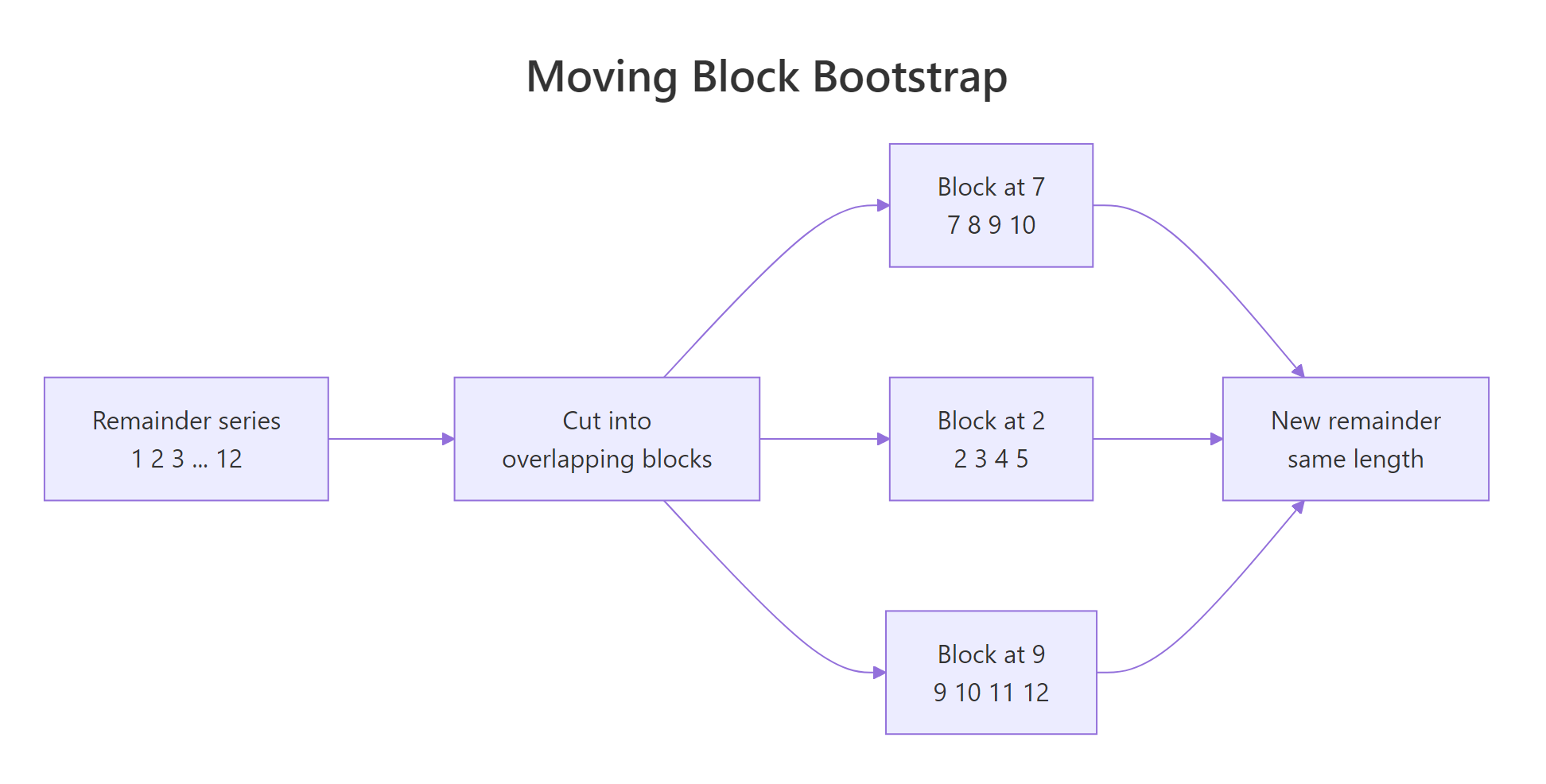
Figure 1: The moving block bootstrap draws runs of consecutive values, so neighbours stay neighbours.
That mechanism is called the moving block bootstrap, and it is easiest to understand on twelve numbers you can read at a glance.
The block length here is 4. sample(1:9, 3, replace = TRUE) picks three starting positions, 1:9 because a block of 4 starting at 10 or later would run off the end. Each start s then grabs small[s:(s+3)], four consecutive values.
Look at the final line. The blocks are in a new order and block 9 was drawn twice, so the series has genuinely been reshuffled. But inside each block, 7 is still followed by 8, which is still followed by 9. The local structure is untouched; only the arrangement of the chunks changed.
The word "moving" refers to the blocks being allowed to start anywhere, not just at fixed cut points. That means blocks overlap, which gives far more distinct blocks to draw from and keeps the manufactured series from looking like a jigsaw of the same few pieces.
Here is the same idea as a reusable function, tested on a series with strong memory built in.
Walking through my_mbb(): it draws two extra blocks beyond what it needs so the concatenated string long is comfortably longer than the original, then trims back to exactly n values starting from a random offset. That random offset is what stops every bootstrap from beginning at a block boundary, which would leave a visible seam pattern.
arima.sim(list(ar = 0.8), n = 200) generates 200 points where each value is 0.8 times the previous one plus fresh noise, a deliberately sticky series. The result is the point of this whole section: block resampling keeps the lag-1 autocorrelation at 0.729 against an original of 0.792, while plain shuffling drops it to -0.068. Blocks preserve the memory; single-point resampling destroys it.
Try it: Run my_mbb() on a fresh AR(1) series twice, once with block_size = 2 and once with block_size = 24, and compare the lag-1 autocorrelations against the original.
Click to reveal solution
Explanation: With blocks of 2, only every other adjacency survives a join, so the recovered autocorrelation falls to 0.374, less than half the original. With blocks of 24, the joins are rare enough that 0.827 comes out essentially identical to the original 0.822.
What are the steps inside bld.mbb.bootstrap()?
Block resampling alone is still not enough. AirPassengers has a rising trend and a repeating yearly wave, and if you block-resample the raw series you will happily paste a 1958 chunk in front of a 1950 chunk and produce a history that jumps backwards. bld.mbb.bootstrap() avoids that by resampling only the part of the series that has no trend or seasonality left in it.

Figure 2: bld.mbb.bootstrap() only resamples the remainder, then puts the series back together.
The name spells out the recipe. BLD stands for Box-Cox and Loess-based Decomposition, MBB for moving block bootstrap. Step one is the Box-Cox transformation.
A Box-Cox transformation raises the series to a power lambda, with lambda = 0 meaning "take logs." BoxCox.lambda() picks the power that makes the seasonal swings the same size throughout, and lower = 0, upper = 1 confines that search to powers between logging and leaving the series alone, which is exactly the range bld.mbb.bootstrap() uses internally. Here it returns 0.0000661, so close to zero that this is effectively a log transform.
The four numbers show why that matters. In raw passenger counts, the last two years swing more than four times as much as the first two, 76.3 against 17.6. After transforming, the two swings are 0.163 and 0.129, near enough the same. Now a chunk of noise cut from 1958 is the right size to paste into 1950.
Step two splits the transformed series into the parts you want to keep and the part you want to resample.
stl() is Seasonal and Trend decomposition using Loess. It slides a smoother along the series to extract a slow-moving trend, averages each calendar month to extract a repeating seasonal pattern, and calls whatever is left over the remainder. The argument s.window = "periodic" forces the seasonal pattern to be identical every year.
The second output is the sanity check: the three components add back up to the transformed series, 4.7192 for January 1949. Decomposition splits, it does not lose anything.
The remainder is the only piece with no trend and no seasonality left in it, which makes it the only piece that is safe to shuffle. Step three does exactly that and then reassembles.
The line does three things at once. my_mbb(..., 24) block-resamples the remainder using blocks of 24 months, which is two full seasonal cycles. Adding trend and seasonal back puts the structure in. InvBoxCox() undoes the transformation so the numbers are passenger counts again.
That is a complete bootstrap series, built from scratch, and it is what bld.mbb.bootstrap() returned in the very first code block. The monthly values differ from the original by a few passengers each, but the twelve-year mean lands at 279.6 against the real 280.3. The manufactured history is different in its details and identical in its character.
Try it: Rebuild one more bootstrap series using blocks of 12 months instead of 24, store it in ex_rebuilt, and compare its overall mean against the original's.
Click to reveal solution
Explanation: Only the block size changed. The rebuilt mean of 281.2 sits within one passenger of the original 280.3, because trend and seasonality were added back untouched and only the small remainder was rearranged.
How do you turn many series into one better forecast?
Now the payoff. You have a machine that turns one history into many. Fit a forecast to each one and average the answers, and you get a forecast that does not hinge on the quirks of the single history you happened to observe. That averaging step is called bagging, short for bootstrap aggregating.

Figure 3: Bagging fits one model per bootstrap history and averages the point forecasts.
To be able to check the result honestly later, split the data first: fit on 1949 to 1958 and hold back the last two years.
ets() fits an exponential smoothing state space model, automatically choosing whether the error, trend and seasonal components should be additive or multiplicative. forecast(fit, h = 24)$mean pulls out the 24 monthly point forecasts. sapply() runs that over all twenty bootstrap series, producing a 24-by-20 matrix: one row per future month, one column per bootstrap history.
rowMeans() then collapses each row of twenty predictions into one. The bagged forecast for January 1959 is 359.6, the average of twenty separate opinions about January 1959.
The forecast package packages that whole loop into one function.
baggedETS(y, bootstrapped_series) fits ets() to every series you hand it and stores the twenty fitted models in fit_bag$models. Passing boot_train reuses the exact ensemble from the previous block, which is why the four numbers match to the decimal. Left to itself, baggedETS() would call bld.mbb.bootstrap(y, 100) and build 100 series.
The table() output shows what the ensemble actually chose. Nineteen of the twenty bootstrap histories led ets() to an ETS(M,Ad,M) model, multiplicative error, damped additive trend, multiplicative seasonality. One led it somewhere slightly different. Which model type gets chosen depends on the particular sample, and bootstrapping is what makes that dependence visible.
Even where the model type agrees, the estimated parameters do not.
alpha is the smoothing weight ETS puts on the most recent observation. A high alpha means the model chases the latest value; a low alpha means it trusts the accumulated level instead.
Fitting once to the real data gives 0.746. Across the twenty bootstrap histories, alpha ranges from 0.602 to 0.775, and the ensemble average is 0.706. In other words, that single estimate of 0.746 sits near the top of a range the data cannot really distinguish between. The bagged forecast uses the whole range instead of betting everything on one draw.
If you like the algebra, here is why averaging helps. Suppose each ensemble member's forecast error has variance $\sigma^2$ and any two members' errors correlate at $\rho$. The variance of their average across $n$ members is:
$$\mathrm{Var}(\bar{f}) = \rho\sigma^2 + \frac{1 - \rho}{n}\sigma^2$$
Where:
- $\bar{f}$ = the bagged forecast, the average of $n$ individual forecasts
- $\sigma^2$ = the error variance of any one ensemble member
- $\rho$ = how strongly two members' errors move together
- $n$ = the number of bootstrap series
The second term shrinks toward zero as $n$ grows, and the first term does not. So averaging removes the part of the error that is specific to one draw of the data, and leaves the part every member shares. If you are not interested in the math, skip ahead: the practical rule is that bagging cuts the wobble, not the bias.
Try it: The fcs matrix has one row per future month and one column per bootstrap series. Bag it with the median instead of the mean, store the result in ex_median_bag, and print the first four months of both side by side.
Click to reveal solution
Explanation: apply(fcs, 1, median) applies median() down each row. The two columns agree to within about one passenger because the twenty forecasts are roughly symmetric with no wild outliers. On messier data with one runaway ensemble member, the median would be the safer choice.
Does bagging actually beat a single ETS model?
Everything so far has been mechanism. Now the honest question: does the extra work buy anything? You held back 1959 and 1960, twenty-four months neither model has seen, so you can just score both.
accuracy(forecast, actuals) compares predictions against truth and returns a row of error measures. RMSE is the typical error in passengers, MAPE the typical error as a percentage, and MASE the error relative to a seasonal naive forecast, where anything above 1 means you did worse than simply repeating last year.
The bagged forecast is better on all three. Typical error drops from 72.6 passengers to 52.1, a 28% improvement. MAPE falls from 13.3% to 9.0%. MASE falls from 2.21 to 1.51, meaning both models still trail a seasonal naive benchmark here, but the bagged one trails it by much less.
The reason connects straight back to the previous section. The single fit landed on alpha 0.746, near the top of the plausible range, so it chased the last few noisy months too hard and over-extrapolated. Nineteen of the twenty bootstrap fits landed lower, and averaging pulled the forecast back toward the middle of what the data actually supports.
AirPassengers is encouraging, not proof. The real evidence is Bergmeir, Hyndman and Benitez (2016), who ran bagged ETS across the 1,428 monthly series of the M3 competition and found consistent accuracy improvements over a single ETS fit. That paper is what put this method into the forecast package.Try it: Score the bagged forecast on the first twelve months of the test set only. Slice the forecast with head(fc_bag$mean, 12), rewrap it as a ts starting January 1959, and compare against window(test, end = c(1959, 12)).
Click to reveal solution
Explanation: Over twelve months the bagged RMSE is 34.0 against 52.1 over twenty-four. Forecast error grows with horizon, so a model always looks better when scored on a shorter window. Always compare models over the same horizon.
Why are the intervals from a bagged model not prediction intervals?
This is the part most tutorials skip, and it is the part most likely to embarrass you in front of stakeholders. forecast() on a bagged model returns something that looks exactly like a prediction interval and is not one.
Compare the two tables. The bagged band for January 1959 runs 345.5 to 374.1, a width of 29 passengers, and it is labelled level 100. The ordinary ETS 95% band for the same month runs 319.6 to 371.3, a width of 52. A supposedly 100% interval a little over half the width of a 95% interval is a contradiction, and the source code explains why.
Internally, forecast.baggedModel() sets lower to the minimum and upper to the maximum of the ensemble's point forecasts, then labels the result level 100. So the band answers "how much do my twenty models disagree with each other?" It says nothing about the noise a future month will actually contain, which is the thing a prediction interval is for.
That also explains a detail you can read off the two tables. The bagged lower bound for January 1959, 345.5, is exactly the plain ETS point forecast for that month. Element one of the bootstrap list is the original series, so one of the twenty ensemble members is the ordinary ets(train) fit, and here that member gave the lowest point forecast of the twenty.
To get a real interval, you need the future noise back. Simulate future sample paths from each ensemble member, then pool them all and read off percentiles.
simulate() on a fitted ETS model draws a random future path rather than the average one, so each call returns a different plausible twelve months. Running it ten times per bootstrap series gives 200 paths in total, stacked into a 12-by-200 matrix. apply(paths, 1, quantile, c(0.05, 0.95)) then reads the 5th and 95th percentile across those 200 futures for each month, giving a 90% interval. model = "MAM", damped = FALSE fixes the ETS specification so both approaches use the same model family and the comparison is fair.
Now compare like with like: both intervals below are nominally 90%. The bootstrap band averages 81.6 passengers wide and actually contains 91.7% of the twelve held-out months. The plain ETS band is narrower at 72.6 and contains only 83.3%. Coverage should sit near the nominal 90%, so the bootstrap band is close to honest and the plain one is overconfident.
That is the real argument for the bootstrap here. The standard ETS interval assumes the model form is correct and only accounts for noise. The bootstrap interval also carries the uncertainty about which model and which parameters were right, so it is wider where it should be.
Try it: The paths matrix already holds 200 simulated futures. Pull the 25th and 75th percentiles out of it into ex_quartiles and print the first three months.
Click to reveal solution
Explanation: Only the requested percentiles changed. The 25% to 75% band spans about 21 passengers in January against roughly 55 for the 5% to 95% band, which is what you would expect: half the future outcomes fall in a much tighter range than 90% of them.
How do you bootstrap and bag the tidy way with fable?
Everything above uses the forecast package and base R ts objects. The modern tidyverse equivalent is fable, which works on tsibble objects and expresses the same idea as a pipeline. The advantage shows up when you have many series at once, because a tsibble can hold thousands of them keyed by an identifier and the same code handles all of them.
The |> symbol is R's native pipe: it feeds the value on its left into the first argument of the function on its right, so ap |> model(...) means the same as model(ap, ...). as_tsibble() converts the ts object into a tidy table with one row per time point. model(stl = STL(Passengers)) fits the same STL decomposition you did by hand earlier. generate() then block-bootstraps the remainder and rebuilds, exactly like bld.mbb.bootstrap(), but returns the results stacked in long form with a .rep column identifying which bootstrap each row belongs to.
The .sim column is the manufactured series. Passengers is the original, kept alongside for reference. With times = 10 this table has 1,440 rows, ten copies of the 144-month history.
Because the ten series are stacked with .rep as a key, fable fits all ten models in one call.
Reading the pipeline: select() drops the columns that would confuse the model call, model(ets = ETS(.sim)) fits an ETS to each of the ten simulated series, and forecast(h = 12) produces twelve months ahead for each. as_tibble() drops the distribution column so plain dplyr verbs work, then group_by(Month) |> summarise(mean(.mean)) averages across the ten forecasts for each month.
That last summarise() is the bagging step, written out in full. The forecast package hides it inside baggedETS(); fable leaves it visible, which is why the tidy version is easier to modify. Swap mean for median, or take quantiles instead, and you have changed the aggregation rule with one word.
baggedETS() is the shortest path for a single ts object. But a tsibble keyed by store, region or SKU runs the identical pipeline across every series at once, and that is where the tidy version earns its extra typing.Try it: Generate only 4 bootstrap series instead of 10 into ex_sims, then report how many rows it has and how many distinct values are in its .rep column.
Click to reveal solution
Explanation: AirPassengers has 144 months, so four bootstrap copies stack into 4 times 144 = 576 rows. The .rep column takes the values 1 to 4, which is what makes them separate series rather than one long one.
How do you choose the block size and the number of series?
Two settings control this whole method, and both have defensible defaults you should understand rather than accept blindly. Start with block size, which you can measure directly: block-resample the remainder at several block sizes and check how much of the original autocorrelation survives.
For each candidate block size, this runs my_mbb() fifty times, measures the lag-1 autocorrelation of each result, and averages. The original_acf1 column is the target to hit.
The pattern is clear. A block size of 1 is plain shuffling and recovers nothing, -0.007 against a target of 0.371. By 6 months you recover 0.320, by 24 months 0.361, and going all the way to 48 buys almost nothing more. The curve flattens at two seasonal cycles, which is exactly where bld.mbb.bootstrap() sets its default: 2 * frequency(y), so 24 for monthly data and 8 for quarterly. If the series has no seasonality at all, frequency(y) is 1 and there is no cycle to key the block length to, so the function falls back to 8 months (or half the series length, whichever is smaller).
The second setting is how many bootstrap series to build. More series means a steadier average, and you can watch the steadiness arrive.
For each ensemble size k, this draws k columns from the twenty available, bags them, then repeats 200 times. The standard deviation of those 200 bagged forecasts measures how much your answer would move if you reran the whole thing with a different random seed.
Bagging just two series leaves 7.82 passengers of seed-to-seed wobble. Twenty series cuts that to 2.86. The gain is steep at first and then flattens, which is the $\frac{1-\rho}{n}\sigma^2$ term from earlier doing its work. Roughly, halving the wobble costs four times the compute.
Try it: Add a block size of 36 to the comparison. Build a small table with just block sizes 24 and 36 and report the recovered autocorrelation for each.
Click to reveal solution
Explanation: Going from 24 to 36 months moves recovered autocorrelation from 0.365 to 0.368, a rounding error. Longer blocks also mean fewer distinct blocks to draw from, so the ensemble gets less varied for no measurable gain in structure.
When bagging does not help at all
Bagging is not free and it is not universal. It costs one model fit per bootstrap series, so 100 series means 100 fits, and the payoff depends entirely on how much of your forecast error came from estimation wobble rather than from the model being wrong. Here is a series where it does not pay.
The setup is identical to the AirPassengers test: fit on everything up to 1977, forecast the twelve months of 1978, score against reality. The only difference is the data.
Bagging loses here. RMSE rises from 289.6 to 316.6 and MASE from 0.48 to 0.50. Look at that MASE: the single ETS was already less than half the error of a seasonal naive benchmark, meaning it fit this series extremely well. There was very little estimation wobble to average away, so bagging spent twenty model fits to add a small amount of noise.
The pattern behind both results is the same. USAccDeaths is short, six years of very regular data with a stable July peak. AirPassengers is twelve years with a growing trend and multiplicative seasonality, where the choice of damping and the smoothing weights genuinely matter and a single fit can land badly.
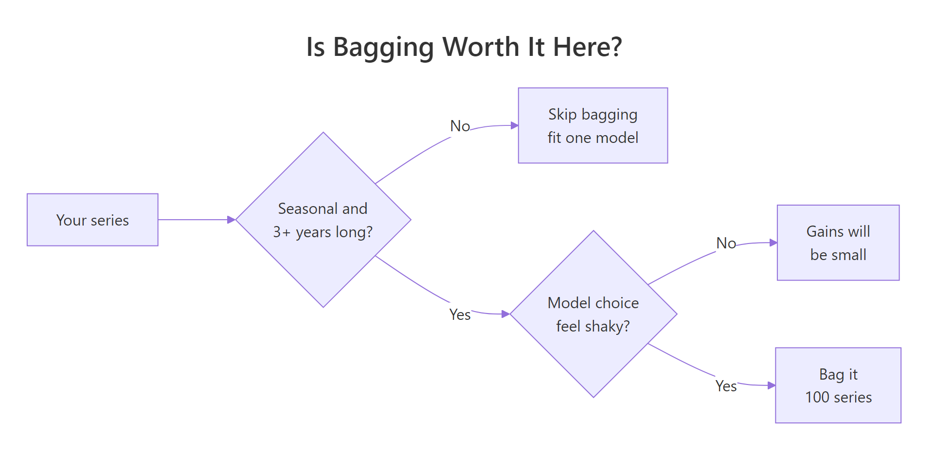
Figure 4: A quick check for whether bagging is likely to pay for its runtime.
Try it: Try a third series. nottem is monthly air temperature at Nottingham Castle from 1920 to 1939. Fit on everything up to 1937, then forecast 24 months and score both approaches.
Click to reveal solution
Explanation: Bagging wins by about 1%, essentially a tie. nottem is temperature data with a rock-solid annual cycle and no trend, so there is almost no ambiguity about the right model and almost nothing for averaging to fix. That is the middle of the three cases: no harm done, no real gain either.
Complete Example: bootstrap, bag, and score in one pass
Here is the whole method wrapped into one reusable function. Hand it a series and a horizon, and it splits, bootstraps, bags, and scores both approaches so you can decide whether bagging earns its runtime on your data.
The function does four things in order. subset() splits the series into a training portion and the last h points held back for scoring. bld.mbb.bootstrap() builds n_boot alternative histories from the training portion only, so nothing from the test period leaks in. Then it fits one plain ets() and one baggedETS(), and accuracy() scores both against the held-back truth.
The numbers reproduce the earlier result exactly, because the same seed produces the same twenty bootstrap series. That reproducibility is the point of the seed argument: rerun it with seed = 999 and the numbers will shift slightly, which tells you how much of any apparent improvement is real and how much is luck. Point this at your own series before committing to bagging in production.
Practice Exercises
Exercise 1: Report the ensemble spread
Write a function my_boot_spread(y, n_boot, h, seed) that bootstraps y into n_boot series, fits ets(s, model = "MAM", damped = FALSE) to each, forecasts h steps, and returns the min, mean and max of the ensemble's forecast for step h. Run it on train with 20 series, h = 1 and seed = 88.
Click to reveal solution
Explanation: sapply() returns one number per bootstrap series, the step-h point forecast. The twenty models disagree by 36 passengers about a single month, from 340.2 to 376.0, which is the estimation uncertainty bagging averages over. This min-to-max range is precisely what forecast.baggedModel() mislabels as a level-100 interval.
Exercise 2: Bag with ARIMA instead of ETS
baggedETS() is a thin wrapper around baggedModel(), which accepts any forecasting function through its fn argument. Build a bagged forecast on train using auto.arima instead of ets, with 10 bootstrap series and set.seed(999), then score it on test.
Click to reveal solution
Explanation: fn = auto.arima swaps the model family without touching the bootstrap machinery, because the bootstrap knows nothing about what will be fitted to its output. Bagged ARIMA scores RMSE 50.67 here, slightly ahead of bagged ETS at 52.06 and well ahead of the single ETS at 72.55. The cost is runtime: auto.arima searches a larger model space than ets, so ten ARIMA fits take longer than twenty ETS fits.
Exercise 3: Measure the coverage of an 80% bootstrap interval
Using the boot_train ensemble already in your session, simulate 10 future paths from each of the 20 bootstrap series (12 months each), extract an 80% interval from the pooled paths, and report both the average width and the share of the twelve held-out months of 1959 that fall inside it. Use set.seed(1500).
Click to reveal solution
Explanation: The 80% band averages 70.0 passengers wide and captures 91.7% of the twelve test months, so it is conservative here: it covers more than the 80% advertised. Twelve months is a small sample, so a single extra hit moves coverage by 8 percentage points. Judging interval quality properly needs many origins, not one.
Frequently asked questions
Is bagging the same as combining different models? No. Combining averages forecasts from genuinely different model families, an ETS plus an ARIMA plus a neural net, on the same data. Bagging averages the same model family fitted to many perturbed copies of the data. Combining targets model-form error; bagging targets estimation error. They stack well together.
How many bootstrap series should I use? Start at the default of 100. The stability table above shows the seed-to-seed wobble falling steeply up to roughly 20 series and then flattening, so anything past 100 buys precision you will not detect in your accuracy metrics while multiplying runtime.
Does this work with ARIMA? Yes. baggedModel(y, fn = auto.arima) swaps the model family while keeping the same bootstrap, and Exercise 2 scores it. The bootstrap does not care what you fit to its output.
Why is the first element returned by bld.mbb.bootstrap() identical to my data? By design. Element one is the original series and elements two onward are bootstraps, so the ensemble always includes the real history. Index from [[2]] if you want only the manufactured ones.
Is it worth the compute? Bagging costs one model fit per bootstrap series. On a single monthly series with 100 replications that is seconds to a minute; across ten thousand SKUs it is an infrastructure decision. Run bag_and_score() on a handful of representative series first and only roll it out where it measurably wins.
Summary
| Concept | Function | The rule |
|---|---|---|
| Plain bootstrap | sample(x, replace = TRUE) |
Fine for independent values, destroys a time series |
| Moving block bootstrap | bld.mbb.bootstrap() |
Resample runs, not points, so autocorrelation survives |
| Variance stabilisation | BoxCox() and BoxCox.lambda() |
Makes early and late noise the same size before resampling |
| Structure quarantine | stl() |
Only the remainder gets shuffled, trend and season are added back |
| Bagging | baggedETS(), baggedModel() |
Average the point forecasts across the ensemble |
| Bagged "interval" | fc$lower, fc$upper |
Ensemble min and max, not a prediction interval |
| Real bootstrap interval | simulate() plus quantile() |
Pool many simulated paths, then read percentiles |
| Tidy equivalent | generate(bootstrap_block_size =) |
Same method in fable, scales to many keyed series |
| Block size | 2 * frequency(y) |
Two seasonal cycles; longer buys nothing measurable |
| Ensemble size | 100 series | Wobble falls like one over the square root of n, then flattens |
| When it pays | Long seasonal series | Big gains where the model choice is genuinely uncertain |
| When it does not | Short clean series | Nothing to average away; fit once and move on |
References
- Bergmeir, C., Hyndman, R. J., and Benitez, J. M. (2016). Bagging Exponential Smoothing Methods using STL Decomposition and Box-Cox Transformation. International Journal of Forecasting, 32(2), 303-312. The paper this method comes from, with the M3 results quoted above. Link
- Hyndman, R. J. and Athanasopoulos, G. Forecasting: Principles and Practice, 3rd edition, Section 12.5: Bootstrapping and bagging. The textbook treatment, in the
fablesyntax used in the tidy section. Link - Hyndman, R. J. and Athanasopoulos, G. Forecasting: Principles and Practice, 2nd edition, Section 11.4. The same material written against
bld.mbb.bootstrap()andbaggedETS(). Link - forecast package reference:
baggedModel()andbaggedETS(). Argument-level documentation, including thefnargument used in Exercise 2. Link - forecast package reference:
bld.mbb.bootstrap(). Where theblock_sizedefault and the returned list structure are documented. Link - Kunsch, H. R. (1989). The Jackknife and the Bootstrap for General Stationary Observations. The Annals of Statistics, 17(3), 1217-1241. The original moving block bootstrap. Link
- Cleveland, R. B., Cleveland, W. S., McRae, J. E., and Terpenning, I. (1990). STL: A Seasonal-Trend Decomposition Procedure Based on Loess. Journal of Official Statistics, 6(1), 3-73. The decomposition that isolates the remainder before any resampling happens. Link
- fabletools reference:
generate.mdl_df(), the tidy bootstrap entry point. Documentstimesandbootstrap_block_size. Link
Continue Learning
- ETS Models in R: Error, Trend, and Seasonal Components explains the model that sits inside every bagged ensemble on this page, and what M, A and Ad actually mean.
- Prediction Intervals in R: Quantify Forecast Uncertainty goes deeper on what a prediction interval is supposed to cover, which is the distinction the bagged interval trap turns on.
- Combining Forecasts in R: Ensemble Averaging covers the other kind of averaging, across different model families rather than across bootstrapped data.