fable in R: Tidy Time Series Forecasting with tsibble
fable is the tidyverse's forecasting package. Your data lives in a tsibble (a table that knows which column is time), you fit any number of models in a single model() call, and you get back tidy tables you can filter, plot and rank like any other data frame. This tutorial builds that whole workflow from scratch, and every code block on this page runs in your browser.
Why does forecasting need its own data structure?
The classic forecasting tools in R take a ts object, which is a plain numeric vector with a start date and a frequency attached to it (the frequency is how many observations make up one cycle, so 12 for monthly data). That works, but it is limiting: a ts can hold only one series, it has no column names, and it stops being a ts the moment you touch it with a dplyr verb like filter(). fable replaces it with a tsibble, a data frame that knows which column is time.
Before explaining any of that, here is the payoff. Three completely different forecasting models, fitted and forecast twelve months ahead, in one pipeline.
Let's walk through what those lines did. AirPassengers is a built-in R dataset counting monthly international airline passengers (in thousands) from 1949 to 1960. as_tsibble() converted it from a ts into a tsibble, and rename() gave the two columns readable names, which is already something you cannot do to a ts. Then model() fitted three models at once and forecast(h = 12) asked each of them for the next twelve months.
Now read the result. The header says A fable: 36 x 4, and 36 is 3 models times 12 months. Every forecast from every model is stacked in one tidy table with a .model column telling you which is which. That is the entire design idea: forecasts are data, so they go in a data frame.
group_by() rather than a pile of bespoke extraction code.Try it: Forecast only six months ahead, using only the SNAIVE model. The starter below fits the model but stops there, so it prints the fitted model instead of a forecast. Add the forecasting step.
Click to reveal solution
Explanation: forecast(h = 6) turns the fitted model into six future rows. SNAIVE just repeats the value from the same month one year earlier, which is why 417 for January 1961 is exactly the January 1960 figure.
What exactly is a tsibble?
A tsibble is a normal data frame plus two pieces of bookkeeping. Almost everything else in this tutorial depends on those two things, so let's name them properly.
The index is the column holding time. Every tsibble has exactly one. The key is zero or more columns that identify which series a row belongs to, for when the table holds several series stacked on top of each other. Everything else is a measured variable, the actual numbers you want to forecast.
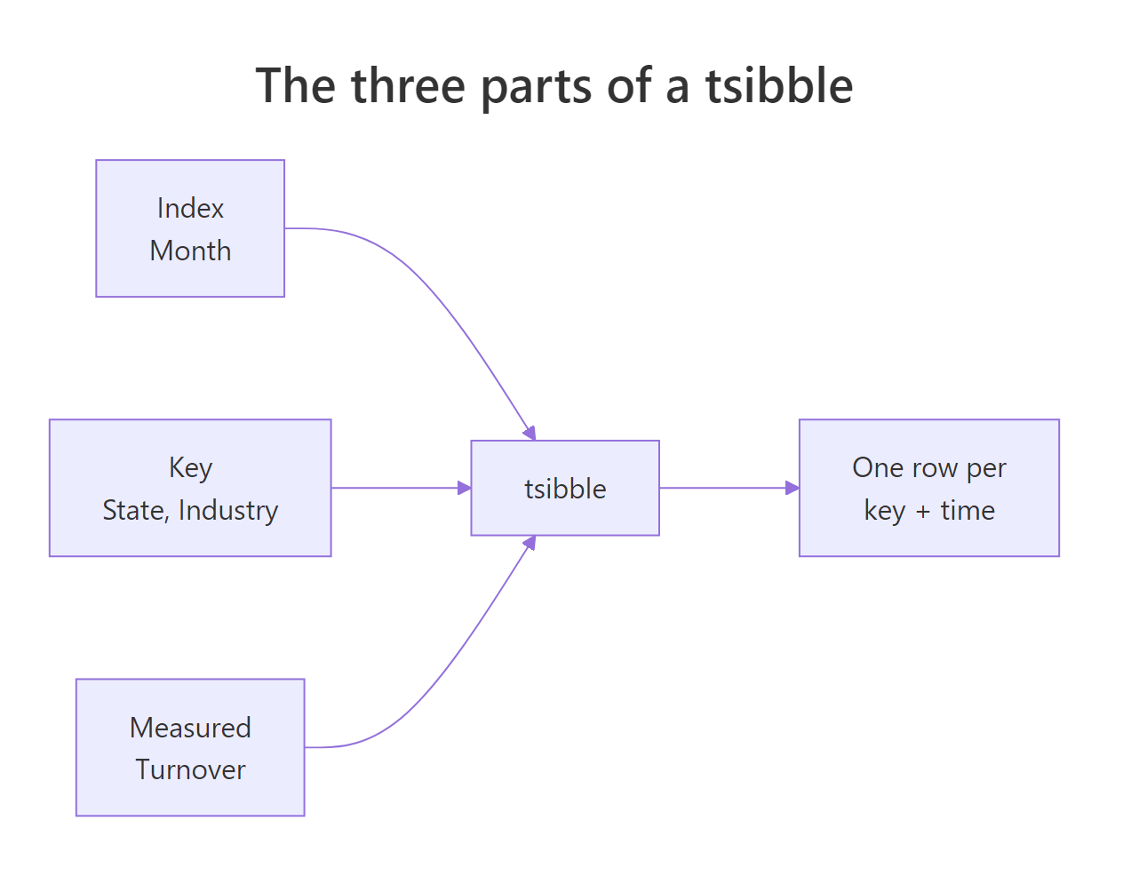
Figure 1: A tsibble wraps an index plus optional keys around the measured values.
The rule that follows from this is simple: index plus key must uniquely identify every row. If you hand tsibble two rows for the same month in the same series, it refuses to build the object rather than silently letting you forecast garbage. Let's look at the tsibble we already made.
The header line carries information a plain tibble would not have. 144 x 2 is the usual rows-by-columns, but [1M] is the interval: one month between observations. fable reads that to know the season is twelve, which is why you never pass a frequency argument anywhere in this tutorial. The <mth> under Month is a year-month type, not a date, so there is no misleading "the 1st of the month" implied.
You can ask the tsibble about itself directly.
index_var() confirms Month is the time column. key_vars() returns character(0), an empty character vector, which means there are no key columns, which means this tsibble holds exactly one series. That is worth remembering, because when we get to forecasting many series at once, the only thing that changes is that this comes back non-empty.
You will not always start from a ts. Most often you have a data frame already, and you promote it with as_tsibble(), or you build one from scratch with tsibble(). Building one from scratch makes the required parts obvious.
Two things to notice. The index = Quarter argument is what makes this a tsibble rather than a tibble, and yearquarter() is what makes the quarters real quarters. The interval in the header came out as [1Q] on its own, inferred from the data.
Because a tsibble is still a data frame, ordinary dplyr verbs work on it. The one genuinely new verb is filter_index(), a shorthand for slicing by time without writing date comparisons.
The ~ reads as "through". You can leave either side open with a dot: . ~ "1958 Dec" means everything up to the end of 1958, and "1959 Jan" ~ . means everything from 1959 onward. We will use exactly that trick to split training data from test data later.
Try it: The starter has three months of website visits as a plain vector, which fable cannot forecast. Turn it into a tsibble with a Month index built by yearmonth() and a Visits column.
Click to reveal solution
Explanation: yearmonth() parses the strings into a month type, and index = Month nominates that column as time. The [1M] in the header confirms tsibble worked out the spacing on its own.
How do you fit ETS, ARIMA and SNAIVE in one call?
Here is where the design starts paying off. model() takes a tsibble and one named argument per model you want, and returns a mable, short for model table. Each column is a model, each row is a series.
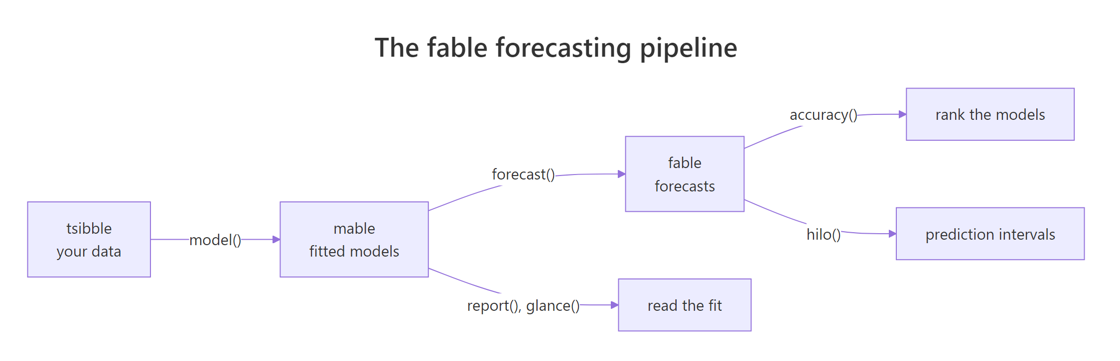
Figure 2: model() turns a tsibble into a mable; forecast() turns a mable into a fable.
The three models we are fitting are worth a sentence each. ETS() is exponential smoothing, which tracks a level, a trend and a season and lets each of them drift. ARIMA() models the series through its own past values and past errors, after differencing, which means replacing each value by its change from the previous one so that a trend is removed. SNAIVE() is the seasonal naive baseline: the forecast for next July is simply last July. That last one is not a serious model, it is the bar every serious model has to clear.
One row, because there is one series. Three columns, because we asked for three models. The interesting part is what is printed inside each cell, because we never specified any model orders. Writing ETS(Passengers) with no further arguments told fable to search the ETS family and keep the best, and it chose ETS(M,Ad,M). Those letters decode as multiplicative errors and a multiplicative season, with an additive damped trend sitting between them. ARIMA(Passengers) ran the same kind of search and landed on ARIMA(2,1,1)(0,1,0)[12]. Read that label as two brackets of three numbers each: the first is the ordinary part, counting past values used, differences taken, and past errors used, so 2, 1 and 1 here. The second bracket is the same three counts applied a whole season apart, so no seasonal past values, one seasonal difference, no seasonal past errors. The trailing [12] says a season is twelve months.
To read one model in full, pull out its column and call report().
Those four smoothing parameters each answer "how fast should this component react to new data", on a scale from 0 to 1. alpha = 0.71 is the level, and it is high, so the level chases recent observations closely. beta = 0.02 is the trend, and it is nearly zero, so the growth rate is treated as almost fixed. gamma = 0.0001 is the season, so the seasonal shape is essentially locked in from the start of the series. phi = 0.98 is the damping, which gently flattens the trend as the forecast goes further out.
When you want to compare all the models at once rather than read one deeply, use glance().
One row per model, with the standard fit statistics. sigma2 is the estimated variance of the errors, log_lik is the log-likelihood, and AIC and BIC are likelihood scores penalised for how many parameters the model spends. SNAIVE shows NA throughout because it is not a likelihood-based model at all, it has nothing to estimate.
Now for a trap. It is tempting to read this table and declare ARIMA the winner because 1018 is a much smaller AIC than 1395. That comparison is not valid. ETS here models the data multiplicatively, so its likelihood is computed on a different scale from the ARIMA one, and AIC values are only comparable between models fitted to the identical response on the identical scale. AIC is for choosing within a family. To choose between families, you need held-out data, which is the next section but one.
Try it: Print the full ARIMA fit, including its coefficients. The starter selects the wrong column and stops short of reporting.
Click to reveal solution
Explanation: Swap ets for arima in select(), then pipe into report(). You get the three fitted coefficients with their standard errors: two autoregressive terms and one moving-average term, matching the (2,1,1) in the label.
What is inside a fable, and why is the forecast a distribution?
forecast() takes a mable and returns a fable, a forecast table. We printed one at the very top of this tutorial, but we skipped over its strangest column. Let's go back and look properly.
The Passengers column has type <dist>, and its first entry reads N(442, 299). That is not a number, it is a whole probability distribution: a normal distribution with mean 442 and variance 299. fable stores the entire forecast distribution for every future time point, and .mean is just a convenience column holding the mean of that distribution, which is the point forecast you would quote.
Watch the variances climb down the column: 299, then 442, then 789, reaching 2205 by October. That is uncertainty compounding with distance. Predicting next month is much easier than predicting ten months out, and the object records exactly how much easier.
Because the distribution is stored rather than a pre-baked interval, you can ask for any interval level you like after the fact with hilo().
A new column named 95% appeared, of type <hilo>, holding the lower and upper bound of each interval. The printout truncates it to keep the table narrow, which is normal.
When you need plain numbers to hand to a spreadsheet or a report, drop the tsibble structure with as_tibble() and select what you want.
The as_tibble() step matters. A fable keeps its key and index structure, so select() would insist on keeping Month and .model even if you asked for just .mean. Converting to an ordinary tibble first lets you take exactly the two columns you want.
fable also plots itself. autoplot() draws the history and the forecast fan in one go, and because the result is a ggplot you can keep adding layers to it.
Passing air as the first argument to autoplot() is what draws the historical line behind the forecasts; without it you would see only the twelve future months floating on their own. The shaded band is the 95 percent interval, and you can see it flare outward with the horizon exactly as the variances predicted.
Try it: Get 80 percent intervals for the ARIMA forecasts only. The starter filters to ARIMA but never asks for intervals.
Click to reveal solution
Explanation: filter() works on a fable like on any data frame, then hilo(level = 80) adds an 80% column. Notice the ARIMA variance for January is 132 against the ETS model's 299, so the ARIMA forecast distribution is much narrower and its 80 percent interval will be correspondingly tighter.
How do you prove which model is actually best?
We have three fitted models and no honest way to rank them yet. AIC cannot compare across families, and SNAIVE does not even have one. The fix is the same as everywhere else in modelling: hide some data, forecast it, then see who came closest.
Time series make this slightly special. You cannot shuffle rows and take a random 80 percent, because that would let the model peek at the future while predicting the past. The split has to be a cut across time, and filter_index() makes that a one-liner.
We kept everything through December 1958 for training, 120 months, and held back the final two years, 24 months, as a test set the models never see. Now refit on the training data only and forecast far enough to cover the whole test period.
Notice what accuracy() was given: the forecasts, and then air, the full dataset. It matches each forecast to the actual value at that month and computes the error. Passing the complete series rather than just test is the usual idiom, and it works because only the overlapping months are scored.
Four error measures are shown, and they answer slightly different questions. RMSE is the square root of the average squared error, in passengers, and squaring gives a large miss much more weight than several small ones. MAE is the average absolute error, also in passengers, and it weights all misses proportionally. MAPE is the average error as a percentage of the actual value, which makes it comparable across series of different sizes but which becomes enormous if any actual value is near zero. MASE is the one that answers the question you probably care about most: it divides the error by the error a naive seasonal forecast would have made on the training data, so MASE below 1 means you beat the naive baseline and above 1 means you did not.
Read the table with that in mind and it says something uncomfortable. ARIMA is clearly best, but its MASE is 1.52, so over a two-year horizon it is still worse than a seasonal naive forecast would have been on this data. Two years is simply a long way to project a growing series.
Now compare that against how the same models looked on the data they were trained on.
The ranking has flipped. On training data ETS wins with an RMSE of 8.90, and both real models look spectacular next to SNAIVE. On held-out data ETS was the worse of the two and its RMSE was eight times larger. Also note SNAIVE's training MASE of exactly 1, which is not a coincidence: MASE is defined against the naive baseline, so the baseline scores exactly 1 by construction.
Try it: The horizon changes the answer. Score the same three models over just six months instead of twenty-four and see who wins.
Click to reveal solution
Explanation: Change h = 24 to h = 6. Now ETS wins, and both real models drop below a MASE of 1, meaning they genuinely beat the naive baseline. The lesson is that "which model is best" is not a property of the data alone, it depends on how far ahead you need to see.
How do you forecast hundreds of series at once?
Everything so far used one series. In practice you rarely have one. You have sales for every product, traffic for every region, demand for every store. This is the part of fable that has no real equivalent in the older tools, and the surprise is how little the code changes.
Remember key_vars(air) returning character(0). Fill that in, and every verb you have already learned starts operating per series automatically. Let's take real retail data with several series in it.
aus_retail is monthly retail turnover in millions of Australian dollars, and we narrowed it to three industries in Victoria. The header now shows the second line we have been waiting for: Key: State, Industry [3]. Two key columns, and [3] distinct combinations, so three series are stacked in these 1,323 rows.
Now fit models. The code is identical to the single-series version.
The mable is now three rows by four columns: two key columns plus two model columns. Six models were fitted and searched for independently, from one line of code that looks exactly like the one-series case. That is what the key column does for you.
Seventy-two forecasts, twelve months for each of six industry-model pairs, and count() works because a fable is a data frame. With 152 series instead of three, the same line would fit 304 models and the code would not change by a character.
Try it: Fit automatic ARIMA models across the three retail series instead of ETS, and look at the orders it picks for each.
Click to reveal solution
Explanation: Each series got its own independent order search. Clothing and department stores landed on the same orders, but liquor retailing came out as (0,1,1)(0,1,2)[12], a different seasonal structure. A single shared model specification would have missed that.
How do you check the residuals before trusting a forecast?
A model that fits well can still be wrong in a way that matters. The check is to look at what the model could not explain, the residuals, and ask whether anything predictable is left in them. If there is, the model has not used all the structure that was in the data, and its prediction intervals are too narrow.
augment() puts the fitted values and residuals back beside the original data.
Three new columns. .fitted is what the model predicted for each historical month, .resid is the plain difference between actual and fitted, and .innov is the innovation residual, the residual on the scale the model actually works in. Those last two differ here because the chosen ETS model is multiplicative: .resid is in passengers, while .innov is a relative error. Always run the diagnostics on .innov, because that is the quantity the model assumes is well behaved.
What should innovations look like? Like noise. No pattern, no relationship between one residual and the next. The Ljung-Box test formalises that by measuring the autocorrelations, meaning the correlation between a residual and the residual a fixed number of months earlier, and asking whether they are jointly larger across a stretch of those lags than chance alone would produce.
We used 24 lags, two full seasonal cycles, which is the usual choice for monthly data. Read lb_pvalue as the probability of seeing this much leftover autocorrelation if the residuals really were noise. Small p-value means the residuals are not noise.
Here all three fail at the 5 percent level. SNAIVE fails by the widest margin, which is expected since it is a baseline that models nothing. ETS fails clearly at p = 0.00095. ARIMA is the closest to passing at p = 0.037, and it was also the model that won on held-out data, which is reassuring, but it still fails.
Be careful about what that means. It does not mean the ARIMA forecasts are useless, and we already measured that they are the most accurate of the three. It means there is still some structure the model has not captured, so its prediction intervals are probably a little too narrow. Treat the point forecasts as usable and the 95 percent intervals as optimistic.
Try it: Innovations should also average out to roughly zero, otherwise the model is biased. Compute the mean and standard deviation of the ARIMA innovations.
Click to reveal solution
Explanation: The mean is 1.34 against a standard deviation of 10.8, so the average error is small relative to the spread but not exactly zero. The model runs very slightly low on average, under-forecasting by about 1.3 thousand passengers a month.
Complete Example: an end-to-end fable workflow
Let's run the whole loop once more on a series we have not touched, to see it as a single piece of work rather than seven lessons. USAccDeaths counts monthly accidental deaths in the United States from 1973 to 1978. The job is to pick a model honestly and then produce a forecast with intervals.
First, hold back the last year, fit the candidates on the rest, and score them on the year we hid.
ETS and ARIMA are effectively tied here, at a MASE just under 0.48, and both comfortably beat SNAIVE at 0.539. All three are below 1, so all three beat the naive baseline, and a MAPE of about 2.7 percent means the typical miss is small. The two leaders split the decision: ETS is fractionally ahead on MASE (0.479 against 0.481) and ARIMA is fractionally ahead on RMSE (289 against 290). A gap that small is noise, so pick on the measure that matters for the job. We will take ARIMA, because RMSE weights the large misses most heavily and a big single-month miss is the expensive kind of error here.
Having chosen, refit on all the data, including the year used for testing, and forecast forward with intervals. Refitting on everything is the right final step: the holdout existed to choose the model, and once chosen you want it trained on every observation you have.
That is the deliverable: 8,336 expected accidental deaths in January 1979, 7,532 in February, with the seasonal dip that February always shows, and a stored distribution behind each one so any interval level is one hilo() away. Five lines, from raw ts to a forecast you can defend.
Practice Exercises
These combine several ideas at once. Each is solvable with only what this tutorial covered. They use my_ variable names so they will not clobber anything from the tutorial above.
Exercise 1: Build a tsibble and forecast it
Convert USAccDeaths into a tsibble with columns named Month and Deaths, fit both an ETS and a SNAIVE model, forecast 12 months, and print the first three ETS point forecasts.
Click to reveal solution
Explanation: rename() after as_tsibble() gives usable names, model() fits both models into one mable, and as_tibble() before select() lets you keep just the two columns you want without the index tagging along.
Exercise 2: Rank three models on a holdout
Using the deaths tsibble from the complete example, train on everything through December 1977, forecast the 12 months of 1978, and produce a table of all three models sorted from best to worst by MASE.
Click to reveal solution
Explanation: The whole evaluation is one pipeline: slice, fit, forecast, score, sort. arrange(MASE) puts the best model first. ETS edges ahead on MASE while ARIMA is fractionally ahead on RMSE, which is a genuine tie and a normal outcome.
Exercise 3: Compare accuracy across two series at once
From aus_retail, take the New South Wales rows for "Liquor retailing" and "Department stores", fit an ETS model to each, and produce a table showing the training RMSE and MASE per industry.
Click to reveal solution
Explanation: Because Industry is a key column, accuracy() reports one row per series without any grouping code. The RMSEs are not comparable between the two industries since they trade at different volumes, but MASE is scale-free, so it is fair to say the liquor series (0.484) is the easier of the two to model.
Frequently Asked Questions
What is the difference between fable and the forecast package? They are by the same author and do much the same statistics. The forecast package works on ts objects and returns a bespoke forecast object per model. fable works on tsibbles, holds many models and many series in one table, and returns tidy data frames. fable is the actively developed successor; forecast is in maintenance.
Can I still use auto.arima()? Not on a tsibble. ARIMA() inside model() is the fable equivalent, and it runs the same style of automatic order search. The main practical difference is that ARIMA() returns a model cell in a mable rather than a standalone object.
What is the difference between a mable and a fable? A mable holds fitted models, one column per model and one row per series. A fable holds forecasts produced from a mable, with a row per model per future time point. model() produces a mable, forecast() turns a mable into a fable.
Why does model() refuse my ts object? fable only accepts tsibbles. Convert first with as_tsibble(), which works directly on a ts, or build one with tsibble() from a data frame. This is deliberate: the tsibble carries the index and key that everything downstream depends on.
What if my series is missing some months? There are two different problems and tsibble separates them. A month that has a row but holds NA in the measured column is an explicit missing value; some models cope with it and others stop with an error, so resolve it before fitting. A month with no row at all is an implicit gap: has_gaps() reports whether any exist and fill_gaps() inserts the absent rows as NA so the series has one row per period again. Check this early, because the interval in the tsibble header, and therefore the seasonal period every model relies on, is inferred from the spacing of the rows.
How do I get plain numbers out of a fable? Pipe through as_tibble() first, then select() the columns you want. The .mean column holds the point forecasts. For intervals, call hilo(level = 95) before converting, which adds a column of lower and upper bounds.
Does fable handle hierarchical forecasting? Yes, through aggregate_key() in tsibble plus the reconciliation functions in fabletools, so forecasts for regions and the national total add up consistently. It builds on everything in this tutorial: the hierarchy is expressed through the key column.
Why did my ETS and ARIMA AICs look so different? AIC is only comparable between models fitted to the same response on the same scale. A multiplicative ETS model and an ARIMA model are not on the same scale, so their AICs cannot be ranked against each other. Use held-out accuracy to compare across model families.
Summary
The tidyverts workflow is three objects and the verbs that move between them. Learn those and the rest is ordinary dplyr.
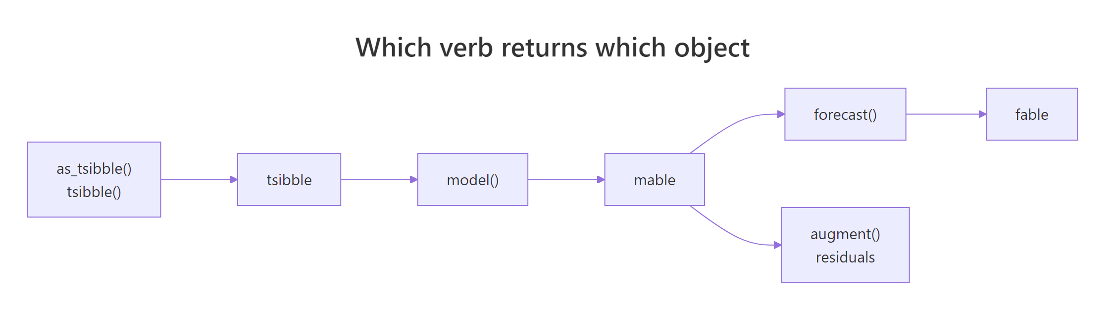
Figure 3: The three objects and the verbs that move between them.
| Object | Made by | What it holds | Read it with |
|---|---|---|---|
| tsibble | as_tsibble(), tsibble() |
Data plus an index and optional keys | index_var(), key_vars(), filter_index() |
| mable | model() |
Fitted models, one column each | report(), glance(), augment() |
| fable | forecast() |
Forecast distributions per model per time | hilo(), accuracy(), autoplot() |
The points worth carrying away:
- The index and key define everything. The index makes seasonality automatic, and the key is the single thing that turns one-series code into many-series code.
- Models live in table cells. That is why
model()fits three models as easily as one, and why comparison is a data frame operation. - Forecasts are distributions, not numbers.
.meanis a convenience; the<dist>column is the real output, which is why any interval level is available after the fact. - Rank models on held-out data only. Our ETS model won on training error and lost badly on the holdout. AIC cannot compare across model families.
- MASE below 1 beats the seasonal naive baseline. It is the one error measure that is both scale-free and honest about whether the modelling was worth it.
- Check
.innov, not.resid. A failed Ljung-Box test means your intervals are too narrow, not that your point forecasts are worthless.
References
- Hyndman, R.J. & Athanasopoulos, G. Forecasting: Principles and Practice, 3rd edition. The definitive text, written around fable. Link
- fable package documentation, tidyverts. Link
- tsibble package documentation: index, key and the tidy temporal data model. Link
- fabletools reference:
model(),forecast(),accuracy()and the mable/fable classes. Link - feasts package: features, decompositions and diagnostics including
ljung_box. Link - Wang, E., Cook, D. & Hyndman, R.J. "A New Tidy Data Structure to Support Exploration and Modeling of Temporal Data", Journal of Computational and Graphical Statistics (2020). Link
- CRAN fable vignette. Link
- Hyndman, R.J. & Koehler, A.B. "Another look at measures of forecast accuracy", International Journal of Forecasting (2006). The paper that introduced MASE. Link
Continue Learning
- ETS Models in R goes deep on the exponential smoothing family, so you can read
ETS(M,Ad,M)and know what each letter changes. - ARIMA Models in R explains differencing, autoregression and moving averages, the machinery behind the
ARIMA()search used above. - Forecast Accuracy in R covers the error measures in more depth, including when MAPE misleads and how to choose a metric for your problem.