Which Forecasting Model in R? A Decision Guide
No single forecasting model wins everywhere. The right choice comes from reading your series' pattern, its trend, its seasonality and its autocorrelation, then shortlisting the models that fit that pattern and backtesting them against a simple baseline so the data, not the hype, picks the winner. This guide walks that process end to end in R, using base R plus the forecast package.
How do you choose a forecasting model in R?
Beginners often ask which model is "the best". That is the wrong question. A model that nails monthly retail sales can fall apart on daily website traffic, and the reverse is just as common. Instead of memorising a winner, you follow a short process: diagnose the pattern, shortlist a few models that suit it, add a naive baseline, then backtest and keep whatever forecasts best.
Here is that idea in action before we unpack it. We take AirPassengers, a classic monthly series of airline passengers from 1949 to 1960, hold out the last two years as a test set, and compare a dead-simple seasonal naive forecast against auto.arima(), which searches for a good ARIMA model on its own.
Read the numbers. The seasonal naive forecast, which just repeats last year's value for the same month, lands a test-set error (RMSE, the typical size of a miss in passengers) of 77.0. The ARIMA model that searched dozens of candidates scores 74.3. That is an improvement of only about three percent. The lesson is not that ARIMA is bad. It is that "advanced" does not automatically mean "better", and the only way to know is to measure on data the model has never seen.
That measure-first mindset is the whole workflow, summarised below.

Figure 1: The four-step model selection workflow, diagnose then shortlist then baseline then backtest.
Try it: Move the split back so the test set is 1958 to 1960, then rerun the same two-model comparison. You will see the ranking can swing a lot with the split, which is exactly why one comparison is never enough.
Click to reveal solution
Explanation: With this split, ARIMA (22.1) beats the baseline (73.6) by a wide margin, far wider than in the main example. The same data with a different split gives a different result. That instability is exactly why we backtest across many origins later instead of trusting one number.
What patterns should you look for in your data?
Before you shortlist any model, you need to know what your series actually does. Three features drive almost every choice: is there a trend (a long-run drift up or down), is there seasonality (a pattern that repeats on a fixed calendar period), and how much autocorrelation is left once you strip those out (how strongly recent values predict the next one).
The cleanest way to see trend and seasonality is to split the series into three parts with STL decomposition: a smooth trend, a repeating seasonal shape and a leftover remainder. We can then measure how dominant each part is. A strength score near 1 means that component explains almost all the variation, and a score near 0 means it is barely there.
Both scores are high. A trend strength of 0.97 says the upward drift is unmistakable, and a seasonal strength of 0.78 says the yearly wave is strong too. So AirPassengers has trend and seasonality together, which already rules out models that handle only one of them and points us toward the seasonal families.
The other question is how much you would have to difference the series to make it stationary, which is what ARIMA needs. Differencing means subtracting the previous value (or the value one season ago) so the level and the seasonal pattern stop drifting. The forecast package can count the differences for you.
The answer is one ordinary difference to kill the trend and one seasonal difference to kill the yearly cycle. That is the classic signature of an airline-style series, and it is exactly what a seasonal ARIMA is built to absorb. If you want the formal hypothesis tests behind stationarity, see the guide on testing stationarity in R.
Try it: The built-in nottem series holds monthly temperatures at Nottingham from 1920 to 1939. Decompose it and compute the strength of seasonality with the same formula. You should land near 0.94, because temperature is almost pure season.
Click to reveal solution
Explanation: A seasonal strength of 0.94 with almost no trend tells you a seasonal model with a flat level, such as seasonal ETS, is the natural first pick for nottem.
Which model matches which pattern?
Once you know the pattern, the shortlist almost writes itself. The decision tree below is the map: start by fitting a naive baseline, then branch on the pattern you found.
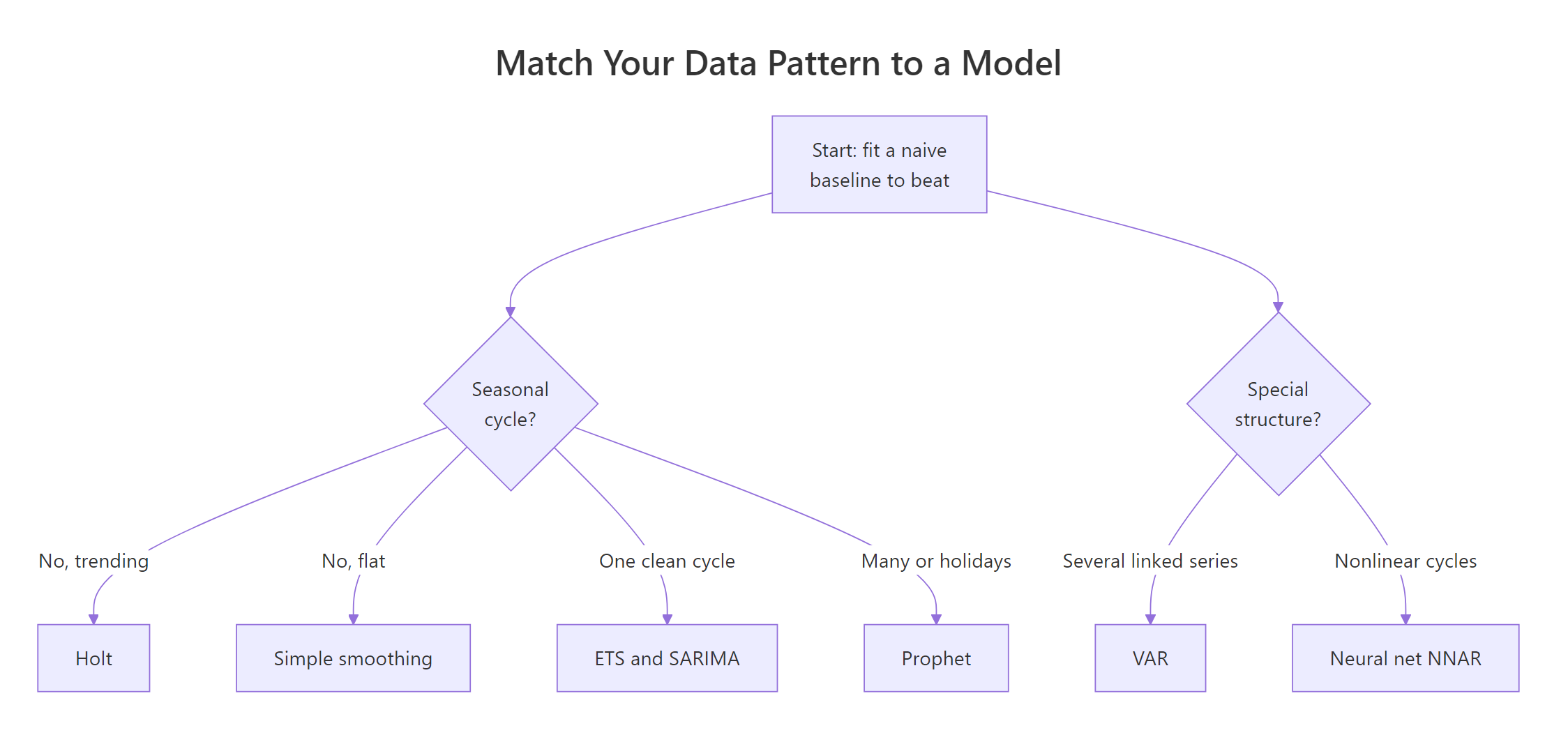
Figure 2: A decision tree from your data's pattern to a candidate model.
Each branch corresponds to a model family. Here is the same map as a lookup table, with the R function that fits each one.
| Data pattern | Model family | R function |
|---|---|---|
| Flat, no trend or season | Simple exponential smoothing | ses() |
| Trend, no season | Holt's linear or damped trend | holt() |
| Trend and one seasonal cycle | ETS or seasonal ARIMA | ets(), auto.arima() |
| Strong autocorrelation and season | Seasonal ARIMA (SARIMA) | auto.arima() |
| Multiple seasons or holidays | Prophet | prophet::prophet() |
| Several series that move together | Vector autoregression | vars::VAR() |
| Nonlinear cycles | Neural network autoregression | nnetar() |
The good news is that you rarely set the internal orders by hand. Both ets() and auto.arima() search their own model spaces and return the best fit by an information criterion, a score that balances how well a model fits the data against how many parameters it uses, so a slightly better fit does not win if it costs a lot of extra complexity. Watch ets() read AirPassengers and label the model itself.
The label ETS(M,Ad,M) is a compact description: multiplicative error, an additive damped trend and multiplicative seasonality. In plain terms, ets() noticed the trend and the growing seasonal swing on its own and encoded both. If you want to understand every letter in that code, the ETS models in R guide breaks them down.
When a series drifts but never repeats, you drop the seasonal machinery and use Holt's method, which extends simple smoothing with a trend term. Here is a made-up sales series that climbs steadily with no season, so Holt is the right tool.
The series ends near 246, and Holt projects it forward to 249.4, then 252.1, 254.7 and 257.4, carrying the recent slope into the future. That is what a trend model buys you: a forecast that keeps climbing instead of flattening out.
Try it: Fit ets() to USAccDeaths, the monthly count of accidental deaths in the US from 1973 to 1978, and read off the model string. Predict the trend letter first: this series has a clear season but no lasting drift, so expect the trend component to be none.
Click to reveal solution
Explanation: ETS(A,N,A) means additive error, no trend and additive seasonality. The N confirms the intuition: ets() found a stable level with a repeating seasonal shape and no long-run drift.
How do you shortlist and compare candidates fairly?
Diagnosing the pattern narrows you to two or three candidates. Now you let them compete. The first, quick comparison is a single train and test split: fit each model on the training portion, forecast the horizon you held out, and score the forecasts. The forecast package's accuracy() reports several error measures at once.
Three columns, three verdicts that happen to agree. RMSE and MAE are both average miss sizes in passengers, so lower is better. MAPE is the average miss as a percentage of the actual value, which is handy for comparing across series on different scales. On all three, ets comes out ahead (RMSE 72.55) of both arima (74.25) and the snaive baseline (76.99). Notice this flips the quick pairwise result from the first section, where ARIMA looked slightly better: a different split, a different winner. That fragility is the whole reason we do not stop here.
If you enjoy the underlying definitions, here are the two error measures used above. Skip this box if you are not interested; the code already computed them for you.
$$\text{RMSE} = \sqrt{\frac{1}{h}\sum_{i=1}^{h}\left(y_i - \hat{y}_i\right)^2}$$
$$\text{MAPE} = \frac{100}{h}\sum_{i=1}^{h}\left|\frac{y_i - \hat{y}_i}{y_i}\right|$$
Where:
- $y_i$ is the actual value at step $i$
- $\hat{y}_i$ is the forecast for step $i$
- $h$ is the number of steps in the test set
A single split can still fool you, because it judges each model on one slice of history. The robust fix is time series cross-validation, also called a rolling-origin backtest: forecast one step from an early cutoff, roll the cutoff forward, forecast again, and repeat across the whole series. The forecast package wraps this in tsCV().
Now the verdict is decisive and stable. Averaged over every origin in the series, the seasonal naive forecast is off by about 36.5 passengers one step ahead, while ETS is off by only 14.5. ETS more than halves the baseline error across the whole history, not just one lucky window, so it is the model you would actually deploy for AirPassengers.
Try it: Rerun tsCV() on the seasonal naive method, but forecast 12 months ahead instead of one step. Longer horizons are harder, so expect the RMSE to rise, landing near 37.
Click to reveal solution
Explanation: At a 12-month horizon the seasonal naive RMSE is 37.1, close to its one-step value here because the yearly pattern is so regular. On messier series, the error would grow much faster with the horizon.
When should you reach for Prophet, VAR, or neural nets?
ETS and ARIMA cover most single-series forecasting, but three situations pull you off that main path. Each maps to a branch on the right of the decision tree.
Prophet is worth reaching for when a single series has more than one seasonal cycle at once (say weekly and yearly), when holidays or promotions cause big one-off spikes, or when you have gaps and outliers you would rather not clean by hand. Prophet fits a curve made of a trend plus seasonal and holiday terms, and it exposes plain-language knobs that a non-specialist can tune. It is not part of the interactive runtime here, so you would run it locally with library(prophet). If your series is a clean single season, Prophet usually offers no accuracy edge over ETS or SARIMA, so do not reach for it by default.
Neural network autoregression suits series whose ups and downs are nonlinear, meaning the jump to the next value is not a straight-line function of the recent past. The nnetar() function fits a small neural net that predicts each value from its own lags, and it runs right here. The lynx series, annual counts of trapped Canada lynx, has famously sharp, irregular boom-and-bust cycles that trip up linear models.
The label NNAR(8,4) means the net uses the last 8 values as inputs and 4 nodes in a hidden layer, and it averages 20 such networks to steady the forecast. We set a seed first because the networks start from random weights, so the seed makes the result reproducible. Neural nets need plenty of history and offer little interpretability, so treat them as a specialist tool, not a default.
Vector autoregression (VAR) is the choice when you have several series that influence each other, and you want to forecast them jointly rather than one at a time. Interest rates, employment and output, for example, move together, so a model that lets each series depend on the recent past of all the others can beat separate univariate models. VAR lives in the vars package, which runs locally rather than in the browser. The block below picks a sensible lag order for Canada's macroeconomic series, where each criterion votes for how many lags to include.
# The vars package is not part of the browser runtime; run this in
# your own R session (install.packages("vars") first if needed).
library(vars)
data(Canada)
VARselect(Canada, lag.max = 6, type = "const")$selection
#> AIC(n)  HQ(n)  SC(n) FPE(n)
#>      3      2      2      3
The four selection criteria suggest two or three lags, and you would fit VAR(Canada, p = 2) from there. The takeaway is not the exact number but the shape of the decision: when series move together, model them together.
install.packages() and the code runs unchanged in RStudio or any local R session.Try it: Fit nnetar() to sunspot.year, the yearly sunspot counts, a textbook nonlinear cycle. Set a seed first, then read the NNAR order it selects. You should see a slightly larger net than the lynx example.
Click to reveal solution
Explanation: NNAR(9,5) uses the last 9 years as inputs and 5 hidden nodes, a bigger net than lynx because the sunspot cycle is longer and more intricate.
Practice Exercises
These pull the whole workflow together. Each solution runs in the same session, so the earlier objects and libraries are still loaded.
Exercise 1: Pick a model for USAccDeaths
Hold out the last 12 months of USAccDeaths as a test set. Fit snaive(), ets() and auto.arima() on the rest, then compare their test-set RMSE and decide which to ship.
Click to reveal solution
Explanation: ARIMA (288.8) and ETS (289.6) are neck and neck and both clear the seasonal naive baseline (341.2). With the two close, you would confirm the pick with tsCV() before deciding.
Exercise 2: Diagnose co2 and name the family
The co2 series is the monthly Mauna Loa carbon dioxide reading. Decompose it, compute the strength of trend and of seasonality, then use the decision tree to name the model family those numbers point to.
Click to reveal solution
Explanation: Trend strength 1.00 and seasonal strength 0.98 mean strong trend with strong season, which is the "trend and one seasonal cycle" branch: fit ETS and seasonal ARIMA, then backtest.
Exercise 3: Write a reusable backtest helper
Turn the train-test comparison into a function test_rmse(y, h) that holds out the last h points of any series y, fits snaive() and ets() on the rest, and returns both test-set RMSEs. Then call it on USAccDeaths with h = 12.
Click to reveal solution
Explanation: Wrapping the split in a function lets you rerun the same fair comparison on any series with one call, which is how you keep model selection consistent across a whole project.
Frequently Asked Questions
What is the single best forecasting model in R?
There is not one. The "no free lunch" idea applies squarely to forecasting: a model that wins on one series can lose on another. The reliable move is to shortlist by pattern and let a backtest decide, which is why ets() and auto.arima() plus a naive baseline are such a common starting trio.
Should I use ETS or ARIMA?
Try both and compare. They overlap but are not identical: some ETS models have no ARIMA equivalent and vice versa. On strongly seasonal data they often finish close, so a rolling-origin backtest usually settles it. The ETS vs ARIMA in R guide runs that head-to-head in detail.
Do I need to make my series stationary first?
Only for ARIMA, and even then auto.arima() handles the differencing for you after ndiffs() and nsdiffs() estimate how much is needed. ETS, Holt and Prophet do not require stationarity, so this is an ARIMA-specific step rather than a universal one.
How much data do I need before a fancy model is worth it?
Rough guidance: you want at least a few full seasonal cycles, so two to three years of monthly data at a minimum before seasonal models are stable. With only a handful of points, a naive or simple smoothing forecast is often the honest choice, and neural nets in particular need long histories.
Is Prophet always the right pick for business forecasting?
No. Prophet shines with multiple seasonalities, holiday effects and messy gaps, but on a clean single-season series it rarely beats ETS or SARIMA. Reach for it when its specific strengths match your data, not by default.
How many models should I compare?
Two or three that fit the diagnosed pattern, plus a baseline. Testing more than that risks picking a winner by chance, so keep the shortlist small and judge it with cross-validation rather than a single split.
Summary
Choosing a forecasting model is a repeatable process, not a lookup of the "best" algorithm. Diagnose the pattern, shortlist the models that fit it, keep a naive baseline as the bar, then backtest and deploy whatever forecasts best on data it has not seen.
| Data pattern | Start with | Confirm by |
|---|---|---|
| Flat level | ses() |
Beat naive() on a backtest |
| Trend, no season | holt() |
Backtest damped vs linear trend |
| Trend and season | ets(), auto.arima() |
Rolling-origin tsCV() |
| Multiple seasons or holidays | Prophet (local) | Compare to ETS or SARIMA |
| Several linked series | vars::VAR() (local) |
Compare to per-series models |
| Nonlinear cycles | nnetar() |
Backtest against a linear model |
The four-step checklist to keep on hand:
- Diagnose trend, seasonality and leftover autocorrelation with
stl(),ndiffs()andnsdiffs(). - Shortlist two or three models from the decision tree that match the pattern.
- Baseline every candidate against
snaive()ornaive(). - Backtest with
tsCV()and keep the model with the lowest rolling-origin error.
References
- Hyndman, R.J. and Athanasopoulos, G. Forecasting: Principles and Practice (3rd ed). Link
- Hyndman and Athanasopoulos. Time series cross-validation, FPP3. Link
- Hyndman, R.J. forecast package reference. Link
- forecast package on CRAN. Link
- fable package documentation. Link
- Prophet documentation, Meta. Link
- vars package on CRAN. Link
Continue Learning
- ETS vs ARIMA in R: the head-to-head comparison of the two workhorse families, run on real data.
- ETS Models in R: what every letter in a label like
ETS(M,Ad,M)means and howets()chooses. - Test Stationarity in R: the formal tests behind the differencing that ARIMA relies on.