Visualize Time Series in R: autoplot(), Seasonal, Lag Plots
Plotting is the first thing you do to a time series and the last thing you should skip. Four plots answer almost every question you will have about a series before you fit anything: the time plot (autoplot()) shows trend, the season plot (ggseasonplot()) shows the shape of a repeating cycle, the subseries plot (ggsubseriesplot()) shows what each month does on its own, and the lag plot with the ACF (gglagplot(), ggAcf()) show whether the series remembers its own past. This post builds all four on one real dataset, explaining every line and every symbol as it goes.
Everything here assumes you can write basic R and that you have met the ts object before. If "monthly ts with frequency 12" is not yet a familiar phrase, read Time Series Objects in R first and come back. Nothing else is assumed: ggplot2, seasonality, lags, and autocorrelation are all defined as they come up.
Our running example. Every plot in this post is built from the same 144 numbers: AirPassengers, the monthly total of international airline passengers, in thousands, from January 1949 to December 1960. It ships with base R, so you already have it. In January 1949, 112 thousand people flew. In July 1960, 622 thousand did. Somewhere between those two numbers is a story about growth and summer holidays, and the whole point of this post is that you cannot see that story in the numbers, only in the pictures.
What does a time plot show that a summary table cannot?
Start with the most ordinary thing an R user does to an unfamiliar variable: summarise it. Then do the one thing that is special about time series data, which is to draw it in time order. The contrast between those two outputs is the entire argument for this post.
The code below loads two packages and produces both. forecast is Rob Hyndman's forecasting package; we use it here purely for its plotting functions, which are built on top of ggplot2. autoplot() is the one-liner: hand it a time series and it draws a time plot, meaning observations on the vertical axis, time on the horizontal axis, joined by a line in the order the observations happened. The + labs(...) part is ggplot2's way of setting the title and axis labels; the + adds a layer to the plot, and labs is short for labels.
Look at what each one told you.
The summary table says: the smallest month had 104 thousand passengers, the largest had 622, the average was 280, and half the months fell between 180 and 361. That is everything a summary can know. It is a perfectly good description of 144 numbers in a bag. Notice what is missing: the table would be identical if you shuffled the 144 months into random order. Every number in it survives shuffling, which is another way of saying that the table cannot see time at all.
The time plot says something the table structurally cannot. Run it and you will see a line that does three things at once. First, it climbs steadily from around 120 in 1949 to around 500 by 1960: that upward drift is called the trend, the long-run direction of the series once you ignore the wiggles. Second, the line is not smooth: it makes the same up-and-down shape every single year, a big hump in the middle of each year with dips at both ends. A pattern that repeats on a fixed, known period like this is called seasonality. Third, those yearly humps get taller as the years go by: the wiggle in 1949 spans a few tens of thousands of passengers, while the wiggle in 1960 spans a couple of hundred thousand.
Trend, seasonality, and swings that grow. Three findings, one line of code, and not one of them is visible in the summary table. That is the payoff, and everything that follows is a way of looking harder at those same three things.
The time plot has one more job, even though AirPassengers gives it nothing to do here. It is where you catch the observations that do not belong. A month sitting far above or below its neighbours is an outlier: a data-entry slip, a strike, a one-off event. The summary table can never show you one, because it absorbs the odd value into the mean and the quartiles and moves on. On a time plot it sticks out and you cannot miss it. The related pattern is a level shift, where the line jumps to a new baseline and simply stays there, which is what an airline merger or a change in how the numbers were recorded looks like. Scan for both before you go any further. Our line has neither, and knowing that is exactly what lets the rest of this post get straight to trend and season.
Note:
autoplot()is not doing anything mysterious. It draws a line from the first observation to the last, in time order, which is the one thing you must never do with data that is not ordered in time. For time series, order is not a detail; it is the whole signal.
Why does autoplot() know how to draw your series?
You gave autoplot() one argument and got a correctly labelled 1949-to-1960 axis, tick marks in years, and a sensible y axis. It never asked you when the data started or how often it was measured. Where did it get that? The answer is worth two minutes, because it explains what autoplot() can and cannot do for you, and it is the reason the rest of the plots in this post are also one-liners.
A ts object is not just a vector of numbers. It is a vector plus two pieces of metadata: when the series starts, and how many observations make up one full cycle. Ask it directly:
Three things to take from that output. frequency() returned 12, which means twelve observations make one full cycle; for monthly data the cycle is a year. This number is what the word seasonal period means, and it is the single most important piece of metadata in the object: it is why R can say "July" instead of "observation 7". start() returned the pair 1949 1, read as "year 1949, month 1". And window() let you ask for a date range in calendar terms rather than by counting positions in a vector, then printed 1949 laid out as a proper calendar row: 112 passengers in January, rising to 148 in July, falling to 104 in November.
Now autoplot(). It is what R calls a generic function: one name that dispatches to different code depending on the class of what you hand it. Give it a ts and it runs the ts method, which reads start and frequency out of the object and builds the year axis from them. Give it a fitted model or a forecast and it runs a different method entirely. You are not calling a plotting function so much as saying "draw this thing appropriately", and the object itself supplies the rest.
Which means the whole trick lives in the object, not the function. Strip the metadata off and watch the plot get dumber:
The numbers are identical, head() confirms it: 112, 118, 132, exactly as before. But the shape of the line is now the only thing left. The x axis counts 1 to 144 with no notion of a year, R cannot label a peak as "July", and every seasonal function later in this post would refuse to run, because with no frequency there is no season to plot. The lesson is practical: if your plots look wrong, suspect the object before you suspect the plotting call. Getting start and frequency right when you build the ts is what buys you every one-liner below.
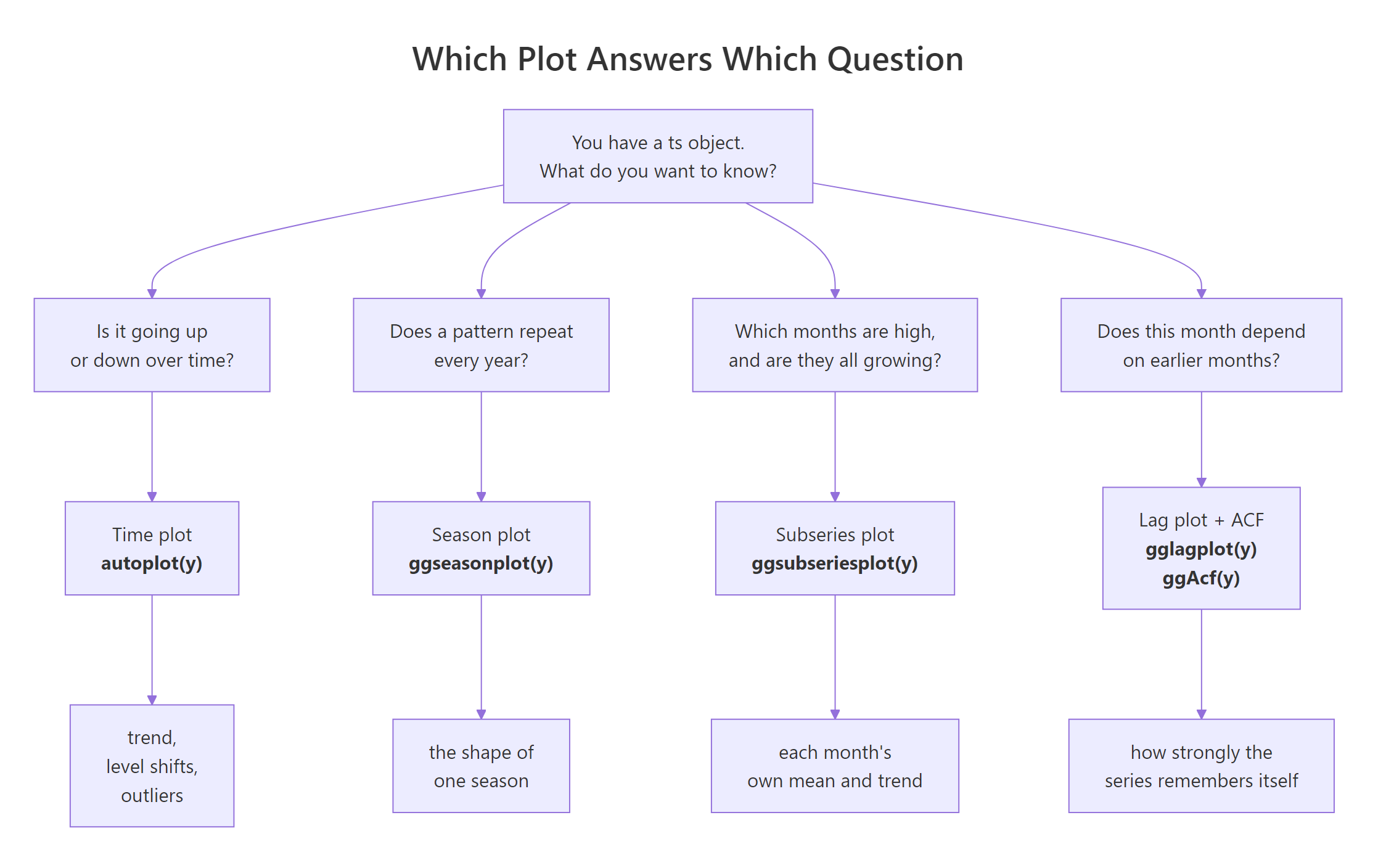
Figure 1: The four questions you can ask a time series, and the plot that answers each. The rest of this post walks the four branches from left to right, all on AirPassengers.
Try it: The series runs to the end of 1960. Plot only the last four years, from January 1957 onward, and check how many months that leaves.
Click to reveal solution
Four years of monthly data is 48 observations, and window() kept the ts metadata intact, so the plot still has a real year axis. Zooming in like this is the standard move when a long series hides its recent behaviour: the seasonal humps that look cramped in the full plot are obvious across four years.
How do you see the season inside the trend?
The time plot told you there is a yearly pattern, but it is hard to study, because the trend keeps dragging the line upward and out of the frame. Every year sits higher than the last, so you are trying to compare shapes that never share a baseline. The fix is a season plot: cut the single long line into one line per year, and stack them all on a common January-to-December axis. The trend becomes vertical separation between the lines, and the seasonal shape becomes the thing they all have in common.
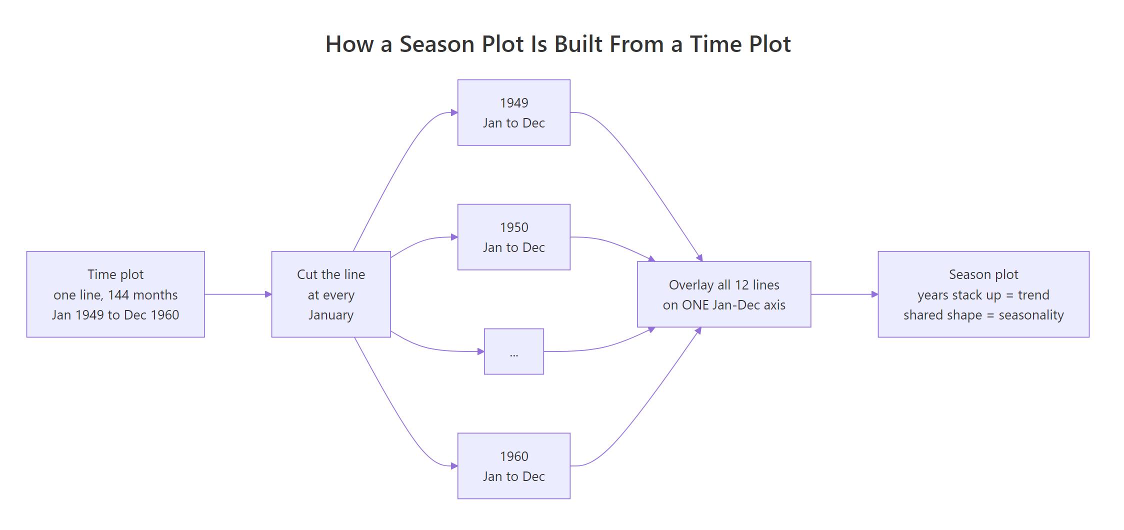
Figure 2: A season plot is the time plot cut at every January and overlaid. Nothing is aggregated or averaged away; the same 144 points are simply re-drawn on a 12-month axis, so 12 years become 12 lines.
ggseasonplot() does the cutting for you, using the frequency from the object to know where a year ends. year.labels = TRUE writes the year at the right end of each line and year.labels.left = TRUE writes it at the left end too, which is what makes it readable at a glance.
The plot shows twelve lines that never cross much: 1949 sits at the bottom, 1960 at the top, and the ten other years stack up in order between them. That neat stacking is the trend, seen from a new angle: later years are higher than earlier years in essentially every month, which is a much stronger statement than "the line goes up". More importantly, all twelve lines share one shape. Each rises into the middle of the year, peaks around July and August, drops sharply into November, and ticks back up in December.
The numbers underneath say the same thing precisely. Averaged over all twelve years, July is the busiest month at 351.3 thousand passengers and August is a whisker behind at 351.1. November is the quietest at 232.8. So the summer peak is worth roughly 118 thousand passengers a month over the November trough, and December's little bump (261.8, up from November's 232.8) is the Christmas travel you would expect to be there.
The tapply() line deserves a walk-through, because it is doing something specific. cycle() takes the ts and returns, for every one of the 144 observations, its position within the cycle: 1 for January, 2 for February, up to 12 for December. tapply(values, groups, mean) then splits the 144 values into those twelve groups and applies mean to each. The result is twelve numbers, one per month, which is exactly the vertical centre of each column of the season plot.
There is a second way to draw the same plot, which sometimes makes the cycle easier to feel:
polar = TRUE bends the January-to-December axis into a circle, so December sits next to January instead of at the opposite end of the page. The spirals grow outward year by year (the trend again) and bulge toward the July side of the circle (the season again). It is the same data as before; the circle just stops the year from having an artificial start and end.
Watch out: A season plot needs a
frequencyabove 1. If you built yourtswithout settingfrequency = 12,ggseasonplot()errors out rather than guessing. That error is almost always a message about the object, not the plot.
Try it: July is the busiest month. Which month is the quietest, and what is its average? Get R to tell you rather than reading it off the plot.
Click to reveal solution
November, at 232.8 thousand passengers on average, is the quietest month of the year. which.min(month_means) returned 11, and month.abb is a base R constant holding "Jan" through "Dec", so indexing it with 11 gives "Nov". Worth noting: November is lower than both October and December, so it is a genuine trough rather than just a point on the way down.
Which months are high, and are they all growing?
The season plot answers "what shape does a year have?" It is much weaker at a related question: "what has July been doing over the twelve years?" To read that off a season plot you have to trace one x position across twelve different lines, which nobody can do accurately. The subseries plot rearranges the same data to make exactly that question easy. It gives each month its own little panel, and inside each panel it draws that month's twelve values as their own mini time plot, in year order, with a horizontal blue line at that month's mean.
Read the plot first. Twelve panels sit side by side, one per month. The blue horizontal lines trace out the seasonal shape you already know: low in the winter months, high in July and August. That much duplicates the season plot. The new information is inside each panel: within every single month, the line climbs from left to right. January rises across the twelve years, and so does February, and so does every other month. No month is shrinking, and no month is flat.
The table makes that precise. In the first six years January averaged 157.2 thousand passengers; in the last six it averaged 326.3, a gain of 169.2. July went from 218.8 to 483.8, a gain of 265.0. Every entry in the growth row is positive, which is the numeric version of "every panel slopes upward". And the row is not flat: July and August gained the most (265.0 and 260.8) while February gained the least (150.7).
The three lines that built that table are worth unpacking, because one of them rests on an assumption you should see. split(values, groups) is the same idea as tapply() from the last section, minus the averaging: instead of collapsing each group down to one number, it hands you the groups themselves. Splitting on cycle(AirPassengers) therefore gives twelve vectors, one per month, and each one holds that month's twelve values in year order, so the seventh vector is July 1949, July 1950, and so on up to July 1960. That ordering is the assumption everything else rests on: it is the only reason x[1:6] means "the first six years" and x[7:12] means "the last six". sapply(by_month, function(x) mean(x[1:6])) then runs that small averaging function across all twelve vectors and simplifies the twelve answers into one named vector, and rbind() stacks the three vectors into the three rows you see printed.
That contrast is the thing the subseries plot is uniquely good at. A time plot mixes trend and season together into one wiggling line. A season plot separates them but makes per-month history hard to read. The subseries plot answers the two questions separately and at once: between panels you read the seasonal pattern (which months are high), and within each panel you read that month's own trend (whether it is growing, and how fast).
Try it: The growth row is measured in thousands of passengers, and July gained the most. But is July really growing faster, or is it just bigger to start with? Compare the months as ratios instead of differences.
Click to reveal solution
Every month roughly doubled, and the ratios sit in a tight band from 1.91 (March) to 2.21 (July). So July's headline gain of 265 thousand versus February's 151 was mostly a story about July being bigger in the first place, not about July growing at a wildly different rate. In differences the months look very unequal; in ratios they look almost the same. That is a hint about the shape of this series, and the next section is about exactly that.
Why do the swings get bigger every year?
Go back to the very first time plot and look at the wiggles rather than the trend. The 1949 hump is small and the 1960 hump is huge. The ratio table you just built says why: the whole series, seasonal swing included, is roughly doubling, not adding a constant. This distinction has a name and a consequence, so it is worth measuring rather than eyeballing.
When the seasonal swing stays roughly the same size no matter what level the series is at, the seasonality is called additive: the season adds a fixed number of passengers. When the swing grows in proportion to the level, it is called multiplicative: the season multiplies the level by a factor. Measure which one AirPassengers is by computing the size of each year's swing, in raw units and as a fraction of that year's smallest month.
The time() function returns the time of each observation as a decimal year, so January 1949 is 1949.000 and February 1949 is 1949.083. Wrapping it in floor() chops off the fraction, leaving just the year, which split() then uses to cut the 144 values into twelve yearly groups.
Now compare the two rows. In raw passengers, the swing grows relentlessly: 44 thousand in 1949, 232 thousand in 1960, more than five times bigger. If the seasonality were additive, that row would be roughly flat. It is not, so it is not additive. As a fraction of the year's own baseline, though, the swing stays in a band from 0.37 to 0.63: the seasonal effect is worth roughly half the quiet month's traffic near the start of the series, and a little more than half near the end. Be honest about that second row, because it is not perfectly flat: it drifts up from an average of 0.47 across the first six years to 0.58 across the last six. But a 1.2-fold rise is nothing next to the raw swing's 5.3-fold one. The swing is mostly keeping up with the level rather than growing under its own steam, and that is multiplicative seasonality, measured rather than asserted.
The standard fix is to take logs. A log turns multiplication into addition (\(\log(a \times b) = \log a + \log b\)), so a swing that multiplies the level becomes a swing that adds a constant on the log scale:
On the log scale the swing sits between 0.32 and 0.49 across twelve years. It keeps the same mild drift the fraction had (0.38 on average across the first six years, 0.46 across the last six), so the log is a good fix rather than a perfect one. But set either of those against 44 climbing to 232 on the raw scale and the difference is the whole point. The plot shows it visually too: the humps are now roughly the same height from one end to the other, and the trend has turned into a near-straight line. That is what people mean by "log-transform to stabilise the variance", and now you have seen the number that justifies it rather than taking it on trust.
Note: The log scale is a viewing choice, not a change to the data. Nothing forces you to model logs just because you plotted them. But if your next step is a model that assumes an additive season (and many do), this plot is how you find out you need the transform, before the model quietly misfits the last three years.
How do you check whether this month depends on last month?
Every plot so far has asked about the calendar: is it going up, does it repeat, which month is high. There is a different kind of question, and it is the one that eventually decides which forecasting model you can use. Does the series remember itself? If July was unusually busy, does that tell you anything about August? If you can predict a month from earlier months, there is structure to exploit. If you cannot, there is nothing there to forecast.
The direct way to look is a lag plot. The lag-\(k\) value of a series is simply the value \(k\) steps earlier, written \(y_{t-k}\); "lag 1" of July is June, "lag 12" of July 1960 is July 1959. A lag plot is a scatter plot of \(y_t\) against \(y_{t-k}\): each point is one month paired with the month \(k\) steps before it. A tight diagonal cloud means "knowing \(y_{t-k}\) tells you a lot about \(y_t\)"; a shapeless blob means it tells you nothing.
lags = 12 asks for twelve panels, one per lag from 1 to 12, and do.lines = FALSE draws points only (the default joins consecutive points, which is unreadable at 144 observations). Colour marks the month, so you can see which part of the year each point came from.
Two panels stand out. Lag 1 is a tight upward diagonal: consecutive months are very similar, which is unsurprising for a series that trends. Lag 12 is also tight, which is the interesting one: what a month looks like is strongly predicted by the same month one year earlier. Lag 6 is the loosest and least diagonal, because a month six away is at the opposite side of the seasonal cycle: summer against winter.
Twelve scatter plots is a lot of looking, though, and we only extracted one number's worth of information from each. That is what the ACF is for. Autocorrelation is the correlation of a series with a lagged copy of itself, and the lag-\(k\) autocorrelation, written \(r_k\), is one number summarising one lag plot:
$$ r_k = \frac{\sum_{t=k+1}^{T} (y_t - \bar{y})(y_{t-k} - \bar{y})}{\sum_{t=1}^{T} (y_t - \bar{y})^2} $$
Every symbol: \(y_t\) is the value at time \(t\); \(T\) is the number of observations (144 here); \(k\) is the lag; \(\bar{y}\) is the mean of the whole series (280.3, from the very first summary). The numerator sums the product of two deviations from the mean: how far above average the series is now, times how far above average it was \(k\) steps ago. When those two tend to have the same sign (both above average, or both below), the products are positive and \(r_k\) is large. The denominator just rescales the whole thing so that \(r_k\) lands between -1 and 1, exactly like an ordinary correlation.
That is a formula, so compute it by hand once and check it against R's answer. Do not take the definition on faith:
The hand calculation gave 0.9480473 and acf() printed 0.948 at the first lag. Same number, so the formula is doing exactly what the words said: y[2:n] is the series from February 1949 onward, y[1:(n-1)] is the same series shifted one month back, and correlating the two is all that \(r_1\) ever was.
One trap in that output. The lags print as 0.0000 0.0833 0.1667 0.2500, not 0 1 2 3. That is because acf() reports lag in units of the seasonal cycle, and for monthly data one month is 1/12 of a year, or 0.0833. So 0.0833 is lag 1 month, not lag 0.08 of anything. ggAcf() labels lags in observations instead, which is why it is easier to read:
Each bar is one \(r_k\), for lags 1 through 36. Two features carry the meaning. The bars start near 0.95 and decay slowly rather than dropping to zero: that slow decay is the signature of a trend, because in a trending series any two nearby months are both high or both low simply by virtue of being late or early. And there are gentle bumps at lags 12, 24, and 36, exactly where the seasonality lives: the same month in earlier years is more correlated than the neighbouring months around it. The blue dashed lines are a significance band, and the next section is about what they actually mean.
Try it: You computed \(r_1\) by hand. Now do \(r_{12}\), the correlation between each month and the same month a year earlier, and check it against acf().
Click to reveal solution
Both give 0.7604. The only change from the \(r_1\) version is the offset: y[13:n] starts at January 1950 and y[1:(n-12)] is the same series shifted back twelve months, so each product pairs a month with its counterpart one year earlier. The $acf component is a vector starting at lag 0, so lag 12 is element 13. Note that 0.7604 is lower than \(r_1\)'s 0.948 even though the seasonal pattern is real and strong; the trend gives every short lag an advantage, which is precisely the effect the next section warns about.
What does a series with no structure look like?
Every plot so far has found something. That is a problem, because you have no idea yet what these plots look like when there is nothing to find, and a chart that always finds a pattern is not evidence of anything. So build the opposite case deliberately: a series that by construction has no trend, no season, and no memory at all. The name for that is white noise, and it is 144 independent random draws with no relationship to each other whatsoever.
rnorm(144, mean = 280, sd = 60) draws 144 independent numbers from a normal distribution centred at 280, deliberately close to the AirPassengers average, and ts(..., start = c(1949, 1), frequency = 12) wraps them up as a monthly series so that R will plot them on the same kind of axis. set.seed(2026) fixes the random draw so your numbers match the ones printed here.
The time plot is the useful shock. It is not a flat line. It jitters up and down, and if you stare at it you will find stretches that look like a rising trend and stretches that look like a dip, because random data does that. This is the single most important calibration in the post: your eye will find patterns in noise. The ACF is what stops it. Almost every bar sits inside the blue dashed band, with no slow decay and no bumps at 12 and 24. Compare it to the AirPassengers ACF from the last section, which started at 0.95 and stayed high for three years, and the difference is not subtle.
That band is a real number, not a decoration. If a series is white noise, each \(r_k\) is a random quantity centred on zero with standard deviation roughly \(1/\sqrt{T}\), so about 95% of them should land within \(\pm 1.96/\sqrt{T}\). The 1.96 is the usual 95% cutoff for a normal distribution, the same number sitting behind any 95% confidence interval. That is where the dashed lines come from, and you can compute them yourself:
The band is 0.163. For the white noise series, 2 of the 36 bars cross it, which is 5.6%, almost exactly the 5% the theory predicts. Those two crossings are not a discovery; they are the price of looking at 36 lags. For AirPassengers, all 36 cross. That is a series drenched in structure.
This is also where the ACF is easiest to over-read, so here is the honest limit of the tool. AirPassengers' huge autocorrelations at lags 20 or 30 do not mean that what happened in August 1955 causes what happens in April 1957. They are mostly the trend: in a series that keeps climbing, any two months are both above the overall mean if they are both late, which the formula reads as correlation. The ACF measures association, and a trend manufactures association at every lag for free. That is why the usual next step is to remove the trend before reading the ACF for model structure, which is the subject of stationarity and differencing.
Watch out: A single bar poking past the dashed line is not a finding. At 36 lags you should expect roughly two crossings from pure chance, which is exactly what the noise series delivered. Read the ACF for its overall shape (slow decay, bumps at the seasonal lag), not for individual bars.
How do the same plots look with tsibble and feasts?
Everything so far used ts objects and the forecast package, which is the classic stack and the reason it works in the code boxes on this page. There is a newer one. tidyverts is a family of packages (tsibble, feasts, fable and friends) that redo time series in tidyverse style, holding the series in a data frame called a tsibble rather than in a ts: Time Series Objects in R covers the difference between the two object types. The plotting functions are near one-to-one with the ones you just learned, so if you have the four questions, you already have this API.
These blocks will not run in the boxes on this page, because the tidyverts packages are not part of this page's runtime. Copy them into your own R session to follow along. The outputs shown are from a real local run on R 4.6.0 with tsibble 1.2.0, feasts 0.5.0, and ggtime 0.2.0.
# install.packages(c("tsibble", "feasts", "ggtime"))
library(tsibble)
library(feasts)
library(ggtime)

air <- as_tsibble(AirPassengers)
air
#> # A tsibble: 144 x 2 [1M]
#>       index value
#>       <mth> <dbl>
#>  1 1949 Jan   112
#>  2 1949 Feb   118
#>  3 1949 Mar   132
#>  4 1949 Apr   129
#>  5 1949 May   121
#>  6 1949 Jun   135
#>  7 1949 Jul   148
#>  8 1949 Aug   148
#>  9 1949 Sep   136
#> 10 1949 Oct   119
#> # ℹ 134 more rows
as_tsibble() converted the ts into a data frame with one row per observation and two columns: index, the month (note the <mth> type, a real month object rather than a string), and value, the passenger count. The [1M] in the header is the tsibble's interval, meaning one month. The metadata that lived invisibly inside the ts is now an actual column you can filter and join on, which is the whole appeal of the format.
The plots then take the tsibble plus the name of the column to plot:
gg_season(air, value)      # season plot   (was ggseasonplot)
gg_subseries(air, value)   # subseries plot (was ggsubseriesplot)
gg_lag(air, value, geom = "point", lags = 1:12)   # lag plot (was gglagplot)
autoplot(ACF(air, value, lag_max = 36))
ACF(air, value, lag_max = 3)
#> # A tsibble: 3 x 2 [1M]
#> lag acf
#> <cf_lag> <dbl>
#> 1 1M 0.948
#> 2 2M 0.876
#> 3 3M 0.807Two things are worth noticing. First, ACF() returns a table, not just a plot: lag 1 is 0.948, lag 2 is 0.876, lag 3 is 0.807, which are the same numbers acf() printed earlier in this post, because it is the same formula. The lags are labelled 1M, 2M, 3M (one month, two months) rather than the confusing 0.0833 the base acf() prints, which is one genuine improvement of the newer stack. Second, the results are in a tidy table you can pipe into filter() or mutate() like any other data frame, instead of being locked in a plot.
Note:
gg_season(),gg_subseries(), andgg_lag()used to live infeastsand moved to theggtimepackage in feasts 0.4.2. Calling them fromfeastsalone still works but prints a deprecation warning, so loadggtimeas shown. If you follow an older tutorial and see that warning, this is why.
Which stack should you use? If you are already in a tidyverse workflow, or your data has multiple series in one table (many products, many stores), tsibble handles that natively where ts does not, and the tidyverts is the better home. If you have one series and want the shortest path from data to picture, ts plus forecast is still perfectly good and is what most existing R material assumes. The plots are the same plots either way; the four questions in Figure 1 do not care which object you store the numbers in.
FAQ
What is the difference between a season plot and a subseries plot? Both re-cut the same series, but along different lines. A season plot draws one line per year on a shared January-to-December axis, so it answers "what shape does a typical year have?" A subseries plot gives each month its own panel containing that month's values across all years, so it answers "what has July been doing over time?" Use the season plot to see the seasonal shape, the subseries plot to see whether individual months are growing or shrinking.
Why does my ggseasonplot() call throw an error? Almost always because the ts has frequency = 1, so there is no season for R to plot. Check with frequency(your_series). If it returns 1, rebuild the object with the right frequency, for example ts(x, start = c(2020, 1), frequency = 12) for monthly data or frequency = 4 for quarterly. The error is about the object, not the plotting call.
Do I need the forecast package just to plot a time series? No. Base R's plot(AirPassengers) gives you a perfectly readable time plot with zero dependencies. What forecast adds is the four-question toolkit as one-liners (ggseasonplot(), ggsubseriesplot(), gglagplot(), ggAcf()) and ggplot2 output you can extend with + labs(), + theme(), and any other layer.
How many lags should I ask for in ggAcf()? A useful default is two to three full seasonal cycles, so lag.max = 24 or 36 for monthly data. That is enough to see whether the seasonal bumps repeat at 12, 24, and 36 rather than being a one-off. Asking for far more lags mostly adds bars that cross the significance band by chance.
The ACF bars are all above the line. Does that mean the series is highly predictable? Not by itself. A trend inflates the autocorrelation at every lag, because in a climbing series any two months are both above the series mean simply for being late in the sample. That is why all 36 AirPassengers bars cross the band. The ACF is most informative about model structure after the trend has been removed, which is what differencing and stationarity testing are for.
Can I use these plots on daily or hourly data? Yes, but ts handles non-integer seasonality badly, and daily data often has two seasonal periods at once (day-of-week and time-of-year). That is one of the strongest arguments for the tsibble and feasts stack, which supports multiple seasonal periods properly; gg_season(air, value, period = "week") lets you pick which one to look at.
Summary
Four plots, four questions, one dataset. Before fitting any model to AirPassengers, the pictures already told us it trends upward, peaks in July, has a multiplicative season worth about half the quiet month's traffic, grows in every month rather than just the summer, and is autocorrelated at every lag out to three years.
| Question | Plot | forecast (ts) | tidyverts (tsibble) |
|---|---|---|---|
| Is it trending? Any outliers? | Time plot | autoplot(y) |
autoplot(y, value) |
| What shape does a year have? | Season plot | ggseasonplot(y) |
gg_season(y, value) |
| Which months are high? Are they growing? | Subseries plot | ggsubseriesplot(y) |
gg_subseries(y, value) |
| Does the series remember itself? | Lag plot | gglagplot(y) |
gg_lag(y, value) |
| How strong is that memory, per lag? | ACF | ggAcf(y) |
ACF(y, value) |
Three things worth carrying forward:
- The metadata does the work.
startandfrequencyare what let every one of these be a one-liner. If a plot looks wrong, inspect the object first. - Growing swings mean multiplicative seasonality. Measure it (swing as a fraction of level, year by year) rather than eyeballing it, and reach for a log when the raw swing climbs but the fraction does not.
- Always have the null in mind. White noise still looks patterned to the human eye. The \(\pm 1.96/\sqrt{T}\) band is the calibration, and roughly 5% of bars cross it for nothing.
Continue with Time Series Objects in R if the ts versus tsibble distinction is still fuzzy, or with Time Series Analysis With R, which picks up where the ACF here leaves off and turns these patterns into models.
References
- Hyndman, R. J. & Athanasopoulos, G. Forecasting: Principles and Practice, 3rd ed., Chapter 2 "Time series graphics". The canonical treatment of exactly these four plots, by the author of the
forecastpackage: otexts.com/fpp3/graphics.html forecastpackage reference. Function-by-function docs forautoplot(),ggseasonplot(),ggsubseriesplot(),gglagplot(), andggAcf(): pkg.robjhyndman.com/forecastfeastspackage site. The tidyverts feature-extraction and statistics package used in the last section: feasts.tidyverts.orgtsibblepackage site. Reference foras_tsibble(), the index/key model, and why intervals matter: tsibble.tidyverts.orgggtimeon CRAN. The new home ofgg_season(),gg_subseries(), andgg_lag()since feasts 0.4.2: cran.r-project.org/package=ggtime- R documentation for
acf(). The exact definition and theplot = FALSEreturn structure used above: stat.ethz.ch/R-manual/R-devel/library/stats/html/acf.html - R documentation for
AirPassengers. Provenance of the running example, from Box, Jenkins & Reinsel: stat.ethz.ch/R-manual/R-devel/library/datasets/html/AirPassengers.html ggplot2reference. For extending any of these plots withlabs(),theme(), and friends: ggplot2.tidyverse.org