Box-Cox and Transformations for Time Series in R

A transformation rewrites a time series on a new scale so that its ups and downs stay roughly the same size from the first observation to the last. In R, BoxCox() applies the whole family of these power transformations, BoxCox.lambda() picks how strong the transformation should be, and passing lambda = to a forecasting function transforms, models and back-transforms in a single step.

Why does a time series need a transformation at all?

Monthly airline passenger counts do something that most real business series do: the peaks and troughs get bigger as the numbers themselves get bigger. That matters, because nearly every forecasting model assumes the size of the wobble stays constant. Here is that problem measured rather than eyeballed, using the gap between the busiest and the quietest month of each year.

Three short steps happened there. time(AirPassengers) returns the decimal date of every observation (1949.000, 1949.083, and so on), and floor() chops that down to a plain year. tapply() then splits the series into those year-sized buckets and runs max(y) - min(y) on each one, which is the distance between December's peak and the quietest month.

Now read the numbers. AirPassengers counts passengers in thousands, so in 1949 the busiest month carried 44 thousand more passengers than the quietest. By 1960 that same gap was 232 thousand, more than five times larger. Nothing about the airline's behaviour changed, the seasonal pattern is exactly as regular as before. The series simply got bigger, and the seasonal swing got bigger with it.

That is a problem for a forecasting model, because a model fits one set of parameters to the whole history. If the wobble in 1960 is five times the wobble in 1949, the model has to compromise: it will overstate the uncertainty in the early years and understate it in the recent ones, which is exactly where your forecast is going to be made.

The fix is not to change the data. It is to change the scale you measure it on. Watch what taking logarithms does to that same picture.

The left panel is a megaphone lying on its side, opening up as it moves right. The right panel is a ribbon of roughly constant thickness that happens to be sloping upward. The trend is still there, the seasonality is still there, and the shape of each year is unchanged. Only the vertical distances have been re-scaled.

Measuring the right panel the same way we measured the left one confirms it.

The gap went from 0.35 to 0.47 over twelve years, a rise of about a third. Compare that with the raw series, where the same gap grew more than fivefold. The log scale has not made the series perfectly uniform, but it has taken an obvious, systematic problem and reduced it to a mild one, which is what a model can cope with.

What does a log transformation actually do?

The log is the transformation you will reach for most often, so it is worth understanding precisely what it fixes rather than treating it as a magic smoother. The one-line version: a log turns multiplication into addition. Anything that is constant in percentage terms becomes constant in absolute terms.

The airline data is a good place to see this, because the seasonal pattern there is multiplicative. December is not "60 passengers above average", it is "26% above average". Let us measure both readings of the same fact.

The two rows describe the same three years, but they tell very different stories. The gap row, which measures the peak in passengers above the yearly average, grows sevenfold. The ratio row, which measures the peak as a multiple of the yearly average, drifts gently from 1.17 to 1.31.

The ratio is the stable description, and that is precisely the quantity a log makes visible, because $\log(a/b) = \log(a) - \log(b)$. Once you take logs, a constant ratio becomes a constant distance, and a constant distance is what an additive model can represent.

The same identity gives you a second, very practical result: the month-to-month difference of a logged series is approximately the growth rate.

diff() subtracts each value from the one after it, so diff(log(x)) gives the change in log passengers from one month to the next. The first entry is 0.0522. The line underneath computes the actual percentage change from January to February the ordinary way, 118/112 minus 1, and gets 0.0536.

Those two numbers, 5.22% and 5.36%, are close but not identical, and the small discrepancy is not an error. A log difference is a continuously compounded growth rate, while the ratio calculation is a simple one. For changes under about 10% the two agree to a decimal place, and the gap widens beyond that. It is a handy reading rule: on a logged chart, a vertical rise of 0.05 means roughly 5% growth.

There is a standard escape hatch for series that touch zero but never go below it: add one before logging, then subtract one when reversing. R ships both halves as a matched pair.

log1p(x) computes log(1 + x), which maps the zeros to zero instead of to negative infinity, and expm1(x) computes exp(x) - 1, which sends everything back exactly where it came from. The round trip in the second line returns the original vector unchanged, which is the property you need: whatever you do to forecast on the transformed scale, you must be able to undo.

Be aware that the "+1" is an arbitrary choice that shifts the whole series, so it changes the fitted model rather than just re-labelling the axis. For a series whose typical value is in the thousands the distortion is negligible. For counts that sit at 0, 1 and 2 it is not, and a count model such as Poisson or negative binomial regression is the better answer there.

What is the Box-Cox transformation, and what does lambda mean?

The log is one fixed amount of squashing. Sometimes it is too much: you take logs and the megaphone flips around, so the swings are now larger at the start of the series than at the end. What you want is a dial rather than a switch, something you can turn up to squash harder or down to squash less, all the way down to no squashing at all.

That dial is the Box-Cox transformation, introduced by George Box and David Cox in 1964. It is a family of power transformations indexed by a single number, $\lambda$ (lambda), that controls the strength.

$$w_t = \begin{cases} \log(y_t) & \text{if } \lambda = 0 \\[4pt] \dfrac{\text{sign}(y_t)\,|y_t|^{\lambda} - 1}{\lambda} & \text{otherwise} \end{cases}$$

Where:

• $y_t$ = the original observation at time $t$
• $w_t$ = the transformed observation at time $t$
• $\lambda$ = the transformation parameter, the dial you set
• $\text{sign}(y_t)$ = +1 for positive values and -1 for negative ones, which lets the formula accept negative values whenever $\lambda > 0$

Two details are worth pausing on. First, the $\lambda = 0$ case is defined separately as the log, which looks like a patch but is not: the limit of the main expression as $\lambda$ approaches zero is exactly $\log(y_t)$, so the family is continuous and the log sits naturally inside it. Second, the subtraction of 1 and the division by $\lambda$ are there to keep the scale sensible and the family continuous. They do not affect which patterns the transformation removes, so if you ever compare against a textbook that uses plain $y^{\lambda}$, the practical behaviour is the same.

Only a handful of $\lambda$ values matter in practice, and it helps to see them as rungs on a ladder.

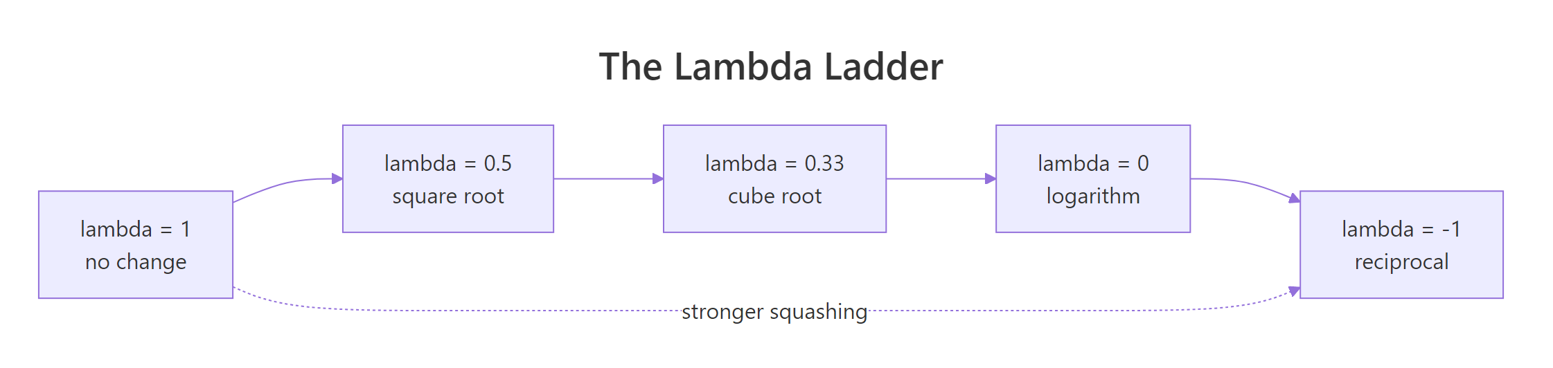
Figure 1: The lambda ladder: one dial from no change to reciprocal.

Reading down the ladder, $\lambda = 1$ leaves the series alone (it just shifts it down by one), $\lambda = 0.5$ takes a square root, $\lambda = 0$ takes a log, and $\lambda = -1$ takes a reciprocal. The further down you go, the harder large values get pulled in relative to small ones.

Now let us actually turn the dial and score the result. We will reuse the yearly-spread measure from the first section, but expressed as a single number: the 1960 spread divided by the 1949 spread. A value of 1 means the swing is the same size at both ends of the series, which is the goal.

BoxCox() from the forecast package applies the formula above at whatever lambda you hand it. The anonymous function transforms the series, computes the yearly spread as before, and returns the last-year-to-first-year ratio. sapply() runs it once per rung of the ladder.

Read the four numbers as a story about over- and under-correction. At $\lambda = 1$ (no transformation) the final swing is 5.27 times the first, which is the fanning we started with. A square root halves the problem to 2.64. The log lands at 1.32, very close to the target of 1. And the reciprocal overshoots badly to 0.33, meaning the swings are now three times bigger at the start of the series than at the end. The megaphone has been flipped around.

Seeing all four at once makes the over-correction obvious.

Top left still fans out. Top right fans out less. Bottom left is the even ribbon we want. Bottom right is visibly worse than bottom left, with the early years now noisier than the late ones. Between 0.5 and -1 there is clearly a sweet spot, and it is somewhere near 0.

One reassurance before we go looking for it: the special case really is the log, not an approximation of it.

Identical to four decimal places, because they are the same operation. This means everything you learned about logs in the previous section, that they turn ratios into distances and that exp() reverses them, carries straight over to the Box-Cox family at $\lambda = 0$.

How do you choose lambda in R?

Turning the dial by hand and looking at plots works, but it does not scale to a hundred series and it is not reproducible. R gives you two automatic methods through a single function, BoxCox.lambda(), and they are worth understanding separately because they can disagree.

The guerrero method, which is the default, is built for exactly the problem we have been measuring. It chops the series into subseries (one per year for monthly data), computes each subseries' standard deviation relative to its own mean, and picks the lambda that makes that relative variability as constant as possible across subseries. In plain terms: it tunes for even swings.

The loglik method takes a different route. It fits a linear regression with a time trend and seasonal dummy variables at each candidate lambda, and picks the lambda that maximises the profile likelihood. In plain terms: it tunes for the value that makes the residuals look most normal.

Let us run both on the airline data.

They disagree, and the disagreement is not small: guerrero picks -0.2947 and loglik picks 0.2000. One says squash harder than a log, the other says squash less. Most tutorials never show you this, which leaves you unprepared the first time it happens on your own data.

The honest interpretation is that both are optimising different things and the objective is flat near its minimum, so the exact number is not very meaningful. What matters is the range. Both answers bracket zero, both are comfortably inside the -1 to 1 window, and both point to "somewhere around a log". You can verify the flatness by sweeping the dial yourself.

The spread_cv column measures how much the twelve yearly spreads vary among themselves, scaled by their average. Lower is better, and zero would mean every year has an identical swing.

The column falls from 0.520 at no transformation to a minimum of 0.091 at $\lambda = -0.25$, then rises again at -0.50. That minimum sits right next to guerrero's -0.2947, which is the confirmation we wanted: guerrero really is optimising for even swings, and our hand-rolled score agrees with it.

But look at how shallow the valley is. Between $\lambda = -0.25$ and $\lambda = 0$ the score moves from 0.091 to 0.137 while the untransformed series sits at 0.520. The difference between "log" and "the optimal lambda" is tiny compared with the difference between "log" and "no transformation at all". The decision that matters is whether to transform, not the third decimal place of lambda.

There is a further reason not to trust the third decimal place: lambda is estimated from your data, so it moves when your data does. Here it is re-estimated on an expanding window, as if you had rerun the analysis every few years.

With only five years of history the estimate is -0.031, which would have told you to use a plain log. Two more years and it drops to -0.269, and from there it settles down near -0.30. The estimate is genuinely unstable on short samples and then stops moving once the series is long enough for guerrero to see the fanning clearly.

That is the honest shape of the situation: lambda is a parameter you estimate, with all the sampling noise that implies, not a physical constant you look up. On five years of monthly data, do not report it to three decimals.

The usual advice that falls out of all this is to let the automatic method tell you the neighbourhood, then round to a simple number in that neighbourhood: 0 for a log, 0.5 for a square root, 1 for nothing at all. Both of our estimates and the manual sweep point at the same neighbourhood here, so $\lambda = 0$ is the natural rounded choice, and it has the advantage of being explainable to a colleague in four words.

Hold that advice loosely, though. It rests on the objective being flat, and flatness in sample does not guarantee that the rounded lambda forecasts as well as the estimated one. We will put exactly that to the test later in this tutorial, and on this series the rounding turns out to cost more than the flat curve above would lead you to expect.

This chart summarises the whole decision.

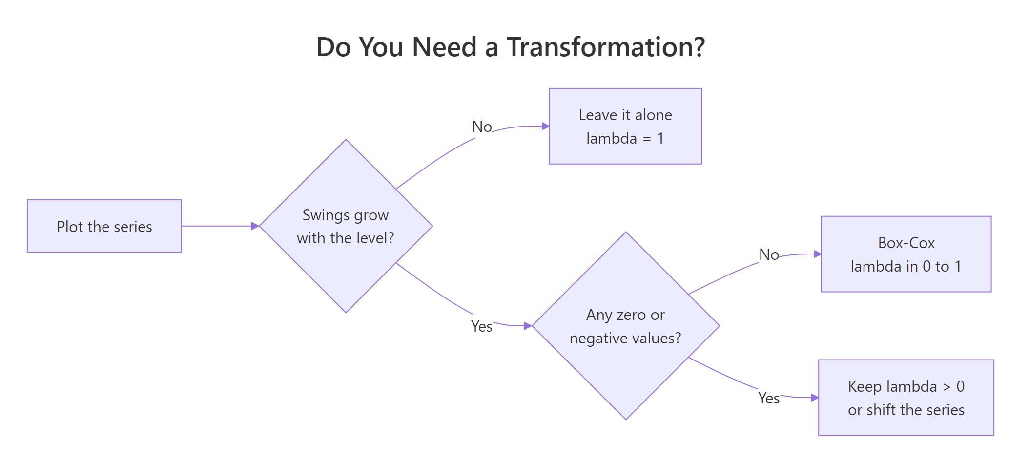
Figure 2: Deciding whether a series needs a transformation at all.

What adjustments should you make before reaching for Box-Cox?

Before you transform anything, it is worth asking whether some of the variability you are seeing is an artefact of how the data was assembled rather than something the business actually did. Three adjustments handle the usual culprits, and all three should happen before a Box-Cox transformation, because they remove a known distortion whereas Box-Cox just re-scales whatever is left.

The first is the calendar adjustment. Monthly totals are contaminated by the fact that months are not the same length. February has 10% fewer days than January, so a monthly total will drop in February even if daily activity is unchanged. Dividing by the number of days converts a total into a daily average, and R has a helper for exactly this.

monthdays() returns the number of days in each month of a monthly time series, correctly handling leap years. Dividing the series by it gives passengers per day, in thousands, rather than passengers per month.

That reframing can flip your reading of a month completely.

On the raw monthly totals, February 1949 looks like a modest 5.4% improvement over January. On a per-day basis it was a 16.7% improvement. Two thirds of the real gain was hidden by February simply being three days shorter. Any model fitted to the raw totals has to learn that calendar effect from scratch, and it will do so imperfectly, whereas dividing by monthdays() removes it exactly and for free.

The second adjustment is for population. If you are forecasting hospital admissions, electricity demand or retail sales for a growing region, part of every upward trend is simply more people. Dividing by population turns the series into a per-capita rate, and what is left is behaviour rather than headcount.

The third is for inflation. Anything measured in currency across many years mixes real change with price change. Dividing by a price index such as CPI and re-basing to a reference year gives you a constant-currency series, so a rise means people bought more, not that the same basket cost more.

How do you forecast on a transformed scale and get back to the original one?

Choosing a transformation is only half the job. Your reader wants a forecast in passengers, not in log passengers, so every transformation has to be reversed before the numbers leave your screen. The reversal has a name and a function: InvBoxCox().

w0 is the log-transformed series we built earlier. Feeding it to InvBoxCox() with the same lambda returns 112, 118 and 132, the original January, February and March 1949 counts. The round trip is exact, which is the property the whole workflow rests on.

The full journey therefore has four legs, and it is worth having the shape of it in your head before we write the code.

Figure 3: Transform, model, back-transform, bias-adjust.

Doing all four by hand is tedious and easy to get wrong, so R's forecasting functions take a lambda argument and handle the whole round trip internally. Let us split the airline data into a training decade and a two-year holdout, then fit a seasonal ARIMA on the log scale.

Reading it in order: window() cuts the series at the end of 1958. Arima() fits the classic airline model, a seasonal ARIMA(0,1,1)(0,1,1), and the lambda = 0 argument tells it to log the data before fitting. forecast() then produces 24 months ahead, and because the model carries its lambda around with it, the output is already back on the passenger scale.

You do not need to know how that ARIMA model works to follow this section. It is held fixed in every comparison below, so the transformation is the only thing that changes.

The point forecast for January 1959 is 348.6 thousand passengers, with an 80% interval running from 332.1 to 365.9. Note that the interval is not symmetric around the point forecast: it extends 16.5 below and 17.3 above. That asymmetry comes from the back-transformation, and it is correct rather than a bug. R computes the interval on the log scale, where it is symmetric, then passes both endpoints back through InvBoxCox(). The exponential curve stretches the upper end more than the lower end, so the interval arrives slightly lopsided, which is the honest shape for a quantity that cannot go below zero.

If you want to see that there is no magic in the lambda argument, here is the same forecast done the long way.

348.6, 331.6, 383.2. Identical to the automatic version, because the automatic version is doing exactly these four steps for you. Use the lambda argument in real work, since it also remembers to back-transform the intervals and the residual diagnostics, which is where hand-rolled code usually goes wrong.

Finally, let us see how the forecast did against the two years we held back.

The blue fan is the forecast with its prediction intervals, and the red line is what actually happened. The red line stays inside the band throughout, and the seasonal peaks line up with the forecast peaks rather than drifting away from them, which is what you hope to see from a model that had the right scale to learn on.

Why is the back-transformed forecast a median rather than a mean?

Here is a subtlety that trips up experienced forecasters, and it is the main reason a transformed forecast can be quietly wrong even when everything above was done correctly.

Think about what a point forecast is. It is a summary of a whole distribution of possible futures. On the log scale that distribution is symmetric, so its mean and its median are the same number and it does not matter which one you report.

Now push that distribution through exp(). The exponential curve stretches the top half more than the bottom half, so the symmetric bell becomes a right-skewed one. The median is unchanged by this, because the middle value is still the middle value no matter how you stretch the axis. The mean is not: stretching the upper half further than the lower half raises the average.

So the number forecast() gives you by default is the median of the back-transformed distribution, not its mean. For many purposes that is fine, but a median is not what you want when the forecast will be added to other forecasts, or compared against an average.

The correction has a formula. For $\lambda = 0$ the bias-adjusted mean is

$$\hat{y}_{T+h|T} = \exp\!\left(\hat{w}_{T+h|T}\right)\left[1 + \frac{\sigma_h^2}{2}\right]$$

and for other lambda values it is

$$\hat{y}_{T+h|T} = \left(\lambda \hat{w}_{T+h|T} + 1\right)^{1/\lambda}\left[1 + \frac{\sigma_h^2(1 - \lambda)}{2\left(\lambda \hat{w}_{T+h|T} + 1\right)^{2}}\right]$$

Where:

• $\hat{y}_{T+h|T}$ = the bias-adjusted forecast for $h$ steps ahead, on the original scale
• $\hat{w}_{T+h|T}$ = the forecast on the transformed scale
• $\sigma_h^2$ = the forecast variance on the transformed scale at horizon $h$
• $\lambda$ = the transformation parameter

The structure of both formulas is the same: take the plain back-transform, then multiply by a correction factor that is always slightly greater than 1. The size of the correction is driven by $\sigma_h^2$, the forecast variance, which grows as you forecast further out. Near-term forecasts barely move, distant ones move more.

If you are not interested in the algebra, skip straight to the code. R applies both formulas for you through a single argument, biasadj.

The cbind() puts the default forecast (a median) beside the bias-adjusted one (a mean) so you can read the gap directly.

At the first horizon the two differ by 0.2 passengers, which nobody would notice. Twenty-four months out they differ by 4.8. The pattern is exactly what the formula predicts: the further ahead you forecast, the larger $\sigma_h^2$ becomes, and the more the mean pulls away from the median.

Just over 1% at two years out. On this series with this model the bias is small, and that is the typical case for a well-behaved log transformation. It gets larger when the forecast variance is larger, which happens with noisier series, longer horizons, or a lambda further from 1.

Does the transformation actually improve the forecast?

Everything so far has argued that transforming should help. A transformation is a modelling choice like any other, so the way to settle it is to score it on data the model never saw. We already have a 1959-1960 holdout, so let us fit the identical model without a transformation and put the three candidates side by side.

Notice the first line of that block. lam_tr is estimated from train alone, not from the full series, because lambda is a parameter fitted from data like any other. Estimating it on all twelve years and then scoring on the last two would let the model peek at its own exam paper, and the resulting accuracy would be flattering rather than informative.

Every row is the same ARIMA(0,1,1)(0,1,1) fitted to the same ten years. The only things that change are the scale it was fitted on and whether the bias adjustment was applied. accuracy() scores each one against the held-out two years on three error measures: RMSE (root mean squared error, in thousands of passengers), MAE (mean absolute error, same units) and MAPE (mean absolute percentage error). Smaller is better on all three.

Start at the top. The untransformed model misses by 72 thousand passengers in a typical month, or 14.4% of the true value. The logged model misses by 43, or 8.5%. That is a 40% reduction in RMSE from a single argument, and it is the main result of this tutorial: on a series whose swings fan out, transforming is not a stylistic preference, it is most of the accuracy.

Row three adds the bias adjustment and shaves off a further 2.6. That improvement is worth a moment's attention. The bias adjustment is not a tuning knob, it is a correction that makes the point forecast mean what it claims to mean, and here it helps accuracy too, because the true series is growing and the median systematically sat below it.

Row four is the uncomfortable one. Swapping our tidy rounded $\lambda = 0$ for guerrero's untidy -0.310 drops RMSE from 40.6 to 27.5, a further 32% improvement, from a change that the in-sample stability curve told us was nearly irrelevant. That curve moved only from 0.137 to 0.091 across the same interval.

So the flat-objective argument is a statement about how the fit responds to lambda, not about how the forecast does. Both things are true at once, and the reason they can diverge is that lambda controls how aggressively the model extrapolates growth: -0.310 squashes the top of the series harder than a log, so the model projected the 1959-1960 growth less steeply, and on this holdout that was the more accurate choice.

The practical resolution is not to abandon rounding, it is to stop treating either choice as settled by theory. Round for explainability when the two score the same, and keep the awkward number when it earns its place on the holdout, which is a decision you can only make by running the comparison above.

Accuracy is only half the scoreboard, though. A forecast also makes a claim about its own uncertainty, and that claim can be checked.

Column 2 of $lower and $upper holds the 95% interval. inside() computes the fraction of the 24 held-out months that landed within the band, and width() computes the band's average height.

The untransformed model's 95% intervals captured the truth only 54% of the time. That is a serious failure: the model was substantially more confident than it had any right to be, because it fitted a single error variance to a decade in which the variance more than doubled. The logged model captured 100%, at the cost of bands that are 22% wider on average.

Neither number is perfect. 100% coverage from a 95% interval on 24 correlated observations suggests the logged bands are, if anything, slightly conservative. But a forecast that is slightly too cautious is a different class of problem from one that is confidently wrong, and only the first one is safe to hand to a planner.

None of this means you should transform everything. When a series already has stable variance, transforming adds a back-transformation step, a bias to worry about and a harder explanation, in exchange for nothing.

Nile records the annual flow of the river at Aswan. Its lambda comes back at 0.999, which is 1 to any reasonable precision, and $\lambda = 1$ means no transformation. That makes sense physically: annual river flow varies around a level rather than growing multiplicatively, so its swings never fanned out in the first place. When the estimate lands on 1, believe it and move on.

Complete Example: the same workflow in fable

The forecast package uses ts objects and function arguments. The newer tidyverts stack (tsibble for the data, fable for the models, feasts for the features) expresses the same ideas as a pipeline, and it puts the transformation directly inside the model formula. Here is the entire workflow in that style, end to end.

The |> symbol is R's native pipe: x |> f() is another way of writing f(x), so each line feeds its result into the next. as_tsibble() converts the ts object into a tidy table with an index column, and rename() gives the value column a meaningful name. The split happens on the next line, before anything is estimated, for the same anti-peeking reason as before. features() then applies the guerrero feature, which is the same estimator we reached through BoxCox.lambda(), and pull() extracts the single number.

It returns -0.3097, matching the forecast-package answer to four decimals. That agreement is the point: these are two interfaces to one statistical method, not two competing methods.

The payoff comes at the modelling step, where the transformation is written into the formula rather than passed as an argument.

Inside model(), ARIMA() searches the order space automatically, and wrapping the response in box_cox(passengers, lam) tells fable to fit on the transformed scale. Left to itself, the search landed on ARIMA(0,1,1)(0,1,1)[12], which is precisely the model we specified by hand earlier. That is a useful reassurance rather than a coincidence: the airline model is called the airline model because it is the right structure for this series.

Because the orders match, whatever difference we see next has to come from the transformation alone.

forecast() returns a distribution that is already back on the passenger scale, because fable keeps the transformation attached to the model rather than leaving it to you. The .mean column is bias-adjusted by default, so you get the mean rather than the median without having to ask for it, which is the opposite of the forecast package's default and a common source of confusion when moving between the two.

Scoring against the full series closes the loop.

RMSE 27.53, identical to the guerrero row of our earlier bake-off, which is exactly what should happen given both stacks fitted the same orders with the same lambda on the same training window. The two ecosystems are interchangeable here; they differ in ergonomics, not in statistics.

Which one you use is a matter of taste and codebase. If you are already writing tidyverse pipelines, fable's formula syntax is harder to get wrong, because the transformation cannot become detached from the model it belongs to, and the bias adjustment is on by default.

Frequently asked questions

Is this the same Box-Cox I learned in regression?

The formula is identical, but the goal is not. In regression you apply Box-Cox to make the residuals closer to normal and homoscedastic, and MASS::boxcox() estimates lambda from a fitted model's likelihood. In time series you apply it to the series itself so that the seasonal and random variation stays the same size over time. The guerrero method exists specifically for the time series goal, which is why it can disagree with a likelihood-based estimate.

Does a Box-Cox transformation make my data normal?

Not reliably, and normality is not what you are after. The transformation is a variance-stabilising tool first; any improvement in symmetry is a side effect. A series can be perfectly variance-stabilised and still have skewed residuals, and models like ARIMA need constant variance far more than they need normality.

What if the automatic lambda comes back negative?

Check two things. First, that the series is strictly positive, since guerrero is only defined for positive data and will warn you otherwise. Second, plot the back-transformed prediction intervals, because negative lambdas stretch the upper tail hard. If the intervals look reasonable, a mildly negative lambda is fine; the airline data's -0.2947 is a perfectly sensible answer. If they explode, round toward 0.

Should I re-estimate lambda inside every cross-validation fold?

Strictly, yes, because lambda is estimated from data and leaking the full sample into an early fold is a mild form of look-ahead bias. In practice, most people estimate lambda once on the training set and hold it fixed, which is defensible given how flat the objective is. What you should not do is estimate lambda on the full series including your test set and then report test accuracy.

If I am already differencing, do I still need a transformation?

Yes, they fix different problems. Differencing removes trend and seasonality, which are patterns in the level. A transformation stabilises the variance. A series can be differenced to stationarity in the mean and still have a variance that doubles across the sample, which is exactly the AirPassengers case. The usual order is transform first, then difference.

Practice Exercises

Exercise 1: Quantify the squash on lynx

The lynx dataset holds annual Canadian lynx trappings from 1821 to 1934, a famously spiky series. Find its guerrero lambda, apply the transformation, and report the standard deviation of the series before and after so you can see how much the transformation compressed it. Save the lambda to ex_lam.

Exercise 2: Run a transformation bake-off on UKgas

Split UKgas into a training set ending in 1984 Q4 and a test set starting in 1985 Q1. Fit the same seasonal ARIMA(0,1,1)(0,1,1) twice, once untransformed and once with a guerrero-chosen lambda, forecast 8 quarters, and compare RMSE and MAPE on the test set. Use the my_ prefix for your variables so you do not disturb the tutorial state.

Exercise 3: Build a bias table across horizons

Using the train series and the airline model with lambda = 0, build a small data frame showing the median forecast, the bias-adjusted mean forecast, and the percentage gap between them at horizons 1, 12 and 24. This is the table you would use to decide whether the bias adjustment matters for your horizon.

Summary

The R functions covered here, and when each one earns its place:

The takeaways in one glance:

• Transform when the swings grow with the level, and measure that rather than eyeballing it: the AirPassengers yearly spread went from 44 to 232 while its logged spread barely moved.
• The log is the workhorse because it turns constant percentages into constant distances, and Box-Cox is the dial that lets you apply more or less of the same medicine.
• Lambda estimates are noisy on short samples, so treat the automatic answer as a neighbourhood rather than a constant, and always pass a proper ts object so the frequency survives.
• Rounding lambda to a tidy 0 buys explainability but is not free: here it cost 32% of the RMSE against the estimated -0.310, so score both rather than assuming the flat in-sample curve settles it.
• Adjust for calendar, population and inflation before transforming, because those distortions can be removed exactly rather than approximately.
• Pass lambda = to the model rather than transforming by hand, so the intervals and diagnostics get back-transformed too.
• The default back-transformed point forecast is a median; set biasadj = TRUE to get the mean, and always do so when forecasts will be aggregated.
• Prove the transformation earned its place on held-out data. Here it cut RMSE by 40% and fixed a 95% interval that was only covering 54% of the truth.

References

1. Hyndman, R.J. & Athanasopoulos, G. - Forecasting: Principles and Practice (3rd ed), "Transformations and adjustments". Link
2. Hyndman, R.J. & Athanasopoulos, G. - Forecasting: Principles and Practice (3rd ed), "Forecasting using transformations", source of the bias-adjustment formulas. Link
3. Box, G.E.P. & Cox, D.R. - "An Analysis of Transformations", Journal of the Royal Statistical Society, Series B, 26(2), 211-252 (1964). The original paper that defined the family and the likelihood method for choosing lambda. Link
4. Guerrero, V.M. - "Time-series analysis supported by power transformations", Journal of Forecasting, 12(1), 37-48 (1993). The paper behind the method = "guerrero" estimator, if you want the subseries argument in full. Link
5. forecast package - BoxCox() and InvBoxCox() reference. Link
6. forecast package - BoxCox.lambda() reference, covering the guerrero and loglik methods. Link
7. feasts package - the guerrero feature for tsibble data. Link
8. fabletools - box_cox() transformation for model formulas. Link
9. R documentation - the AirPassengers dataset. Link

Continue Learning

• Test Stationarity in R - the variance is only half the story, this covers testing and fixing a wandering mean.
• ARIMA Models in R - the model we passed lambda to, explained from the ground up.
• Forecast Accuracy in R - what RMSE, MAE and MAPE really measure, and why they disagreed in Exercise 2.