Test Stationarity in R: ADF, KPSS, and Differencing
A time series is stationary when its statistical behaviour does not depend on when you look at it: same average level, same amount of wobble, same relationship between neighbouring points in 1949 as in 1960. Most forecasting models, ARIMA above all, require this. R gives you two tests that check it from opposite directions: adf.test() asks whether the series has a unit root, and kpss.test() asks whether it is stationary. This post runs both on real data, teaches you to read output that looks contradictory the first time you meet it, and turns the verdict into the only number you actually need: how many times to difference.
Is the airline passenger series stationary?
The series we will use for the whole post is AirPassengers. It ships with R, so you already have it. It holds 144 real numbers: the monthly total of international airline passengers, in thousands, from January 1949 to December 1960. The first month is 112 (meaning 112,000 passengers) and the last is 432.
Two functions do the standard job, both from the tseries package. adf.test() runs the Augmented Dickey-Fuller test. kpss.test() runs the KPSS test. Each prints a test statistic and a p-value.
A test's null hypothesis is the claim it starts out assuming is true and will only abandon if your data makes it look implausible. The p-value measures how implausible: for now, read it the usual way, where below 0.05 means "reject this test's null hypothesis" and above 0.05 means "do not reject it". The catch, and the reason this post exists, is that the two tests have opposite null hypotheses, so the same p-value means opposite things depending on which test printed it.
Here is the whole standard check, on real data.
Read those two results literally and they seem to fight each other.
ADF returned p = 0.01. That is below 0.05, so we reject ADF's null. ADF's null is "the series has a unit root", so rejecting it says: no unit root, this series looks stationary.
KPSS returned p = 0.01. That is also below 0.05, so we reject KPSS's null too. But KPSS's null is "the series is stationary", so rejecting it says: this series is not stationary.
One series, two respected tests, run correctly, and the answers point in opposite directions. Most tutorials never show you this because they pick an example where it does not happen. It happens constantly on real data, and it is not a bug in either test. By the end of this post you will know exactly what causes it, and the answer will make both tests much easier to trust.
You will also see a warning next to each result: p-value smaller than printed p-value. That is normal and worth understanding now so it stops bothering you. Neither test computes p-values from a formula. Both look the test statistic up in a small printed table and interpolate. When your statistic falls off the end of that table, R gives you the nearest edge value and warns that the truth is further out. So p-value = 0.01 from these functions really means "0.01 or less", and (as you will see later) p-value = 0.1 from KPSS really means "0.1 or more". It is a table limit, not an error.
Watch out: The single most common mistake with these tests is reading the p-value without checking which null it belongs to. "p < 0.05, so it's significant, so it's stationary" is right for ADF and exactly backwards for KPSS.
What does "stationary" actually mean?
Before testing for a property, it is worth being able to say what the property is. Informally, a series is stationary if the process generating it has settled down: you could not tell which decade a chunk of it came from by looking at its statistics.
Formally, a series \(y_t\) is (weakly) stationary when all three of these hold:
- Constant mean. \(E[y_t] = \mu\) for every \(t\). The average does not depend on when you measure it. Here \(E[y_t]\) is the expected value (the long-run average) of the series at time \(t\), and \(\mu\) is a single fixed number.
- Constant variance. \(\mathrm{Var}(y_t) = \sigma^2\) for every \(t\). The size of the wobble around the mean does not grow or shrink over time.
- Autocovariance depends only on the gap. \(\mathrm{Cov}(y_t, y_{t+k}) = \gamma_k\), a value that depends on the gap \(k\) but not on \(t\). How strongly today relates to a point \(k\) steps away is the same relationship in 1949 as in 1960.
Notice what is not on that list: the series does not have to be flat, boring or random. It has to be statistically anchored. And notice something else: each of the three rules has a characteristic way of failing. A trend breaks rule 1, because the average keeps moving. Growing swings break rule 2, because the wobble gets bigger. A repeating seasonal pattern breaks rule 1 as well (July's average is not January's average) and shows up in rule 3 too, because points twelve months apart resemble each other more than neighbouring months do.
AirPassengers fails on every count. We do not need a test to see the first two: we can just cut the series in half and compare. One note on how that slicing works. AirPassengers is a ts object, so it carries its own calendar and you cut it by date rather than by position. window() takes a start and an end written as c(year, month), which makes c(1949, 1) January 1949.
The average number of passengers per month roughly doubled, from 182.9 thousand to 377.7 thousand. That kills rule 1. The standard deviation also nearly doubled, from 47.7 to 86.4, so the series does not just sit higher in the 1950s, it swings harder. That kills rule 2. If you had to guess which half a chunk came from, the level alone would tell you almost every time.
The plot says the same thing faster, and you should always look before you test.
You will see a line climbing from 112 up to a peak of 622, with a saw-tooth pattern repeating every year (summer peaks, winter troughs) whose teeth get visibly taller as the line rises. That 622 is July 1960; the 432 we quoted earlier as the final value is December 1960, sitting in the annual trough.
The growing teeth are worth a number of their own. In 1949 the busiest month was 148 and the quietest was 104, a gap of 44. In 1960 the busiest was 622 and the quietest 390, a gap of 232. The annual swing did not merely ride up with the series, it grew more than fivefold.
Three distinct problems in one picture: a rising level, a repeating annual cycle, and swings that grow with the level. Keep that picture in mind, because the rest of the post removes those three problems one at a time.
What is a unit root?
The tests do not actually test the three-rule definition above. They test something narrower and more specific, and understanding it is what makes the ADF output readable.
Start with the simplest interesting model of a series, where each value is a fraction \(\phi\) (the Greek letter phi) of the previous value plus a fresh random shock:
\[ y_t = \phi \, y_{t-1} + \varepsilon_t \]
Here \(y_t\) is the value at time \(t\), \(y_{t-1}\) is the value one step earlier, \(\varepsilon_t\) is a random shock drawn fresh each period with mean zero (think of it as this month's news), and \(\phi\) is a single number that controls how much of the past carries forward. This is called an AR(1) process, short for autoregressive of order 1.
Everything hinges on \(\phi\):
- If \(\lvert \phi \rvert < 1\), the series is stationary. Each shock's influence decays: a shock today is worth \(\phi\) of itself next month, \(\phi^2\) the month after, and so on toward zero. The series has a home level and keeps getting pulled back to it.
- If \(\phi = 1\), the model becomes \(y_t = y_{t-1} + \varepsilon_t\). Every shock is added to the level and never decays. The series has no home to return to, and it wanders forever. This is a random walk, and this case is called a unit root (the "root" of the model equals 1).
That is the whole idea. A unit root means shocks are permanent, which means the series has no fixed mean, which means it is not stationary. A unit root produces what is called a stochastic trend: the series drifts, but the drift is made of accumulated randomness rather than an underlying line.
Let us build both kinds by hand, so we know the right answer before we ask a test for it. This is the single most useful habit when learning a statistical test: run it on data whose truth you control.
One line needs a word of explanation. set.seed(42) pins R's random number generator to a known starting point, so the "random" draws come out the same every time the code runs. That is why the numbers you get will match the numbers printed here exactly, and it is why any of the simulations on this page can be reproduced.
white_noise is 200 independent standard normal draws. It is stationary by construction: fixed mean of 0, fixed variance of 1, no relationship between neighbours. random_walk is cumsum() of a different set of 200 shocks, meaning element 5 is the sum of shocks 1 through 5. That is exactly \(y_t = y_{t-1} + \varepsilon_t\), so it has a unit root by construction. You can see the accumulation in the printed values: the series is at -2.001, then a +0.334 shock takes it to -1.667, then +1.171 takes it to -0.496. Each value is simply the previous one plus whatever the next shock happens to be.
Be careful about what "wanders forever" does and does not mean. The fourth value is 1.564, so this series does cross back over zero, but not because anything pulled it there: a large positive shock happened to arrive. There is no force in the model tugging it home, which is the whole difference. A stationary series returns to its mean because it is built to; a random walk visits zero only by coincidence, and has no reason to stay.
The key point is that these two series are genuinely different in kind, not just in appearance, and we now have one of each with a known answer. Every test from here on gets checked against them.
How does the ADF test work?
The Augmented Dickey-Fuller test asks one question: is \(\phi\) equal to 1? Rather than estimate \(\phi\) directly, it rewrites the model by subtracting \(y_{t-1}\) from both sides. Writing \(\Delta y_t = y_t - y_{t-1}\) for the month-to-month change, the regression adf.test() actually fits is:
\[ \Delta y_t = \alpha + \beta t + \gamma \, y_{t-1} + \sum_{i=1}^{k} \delta_i \, \Delta y_{t-i} + \varepsilon_t \]
Every symbol, in words:
- \(\Delta y_t\) is this period's change, the thing being predicted.
- \(\alpha\) is an intercept (a constant level).
- \(\beta t\) is a straight-line trend term, with \(t\) counting time. Remember this one, it explains the contradiction from section 1.
- \(\gamma\) (gamma) is the coefficient of interest, and it equals \(\phi - 1\).
- The sum of \(\delta_i \Delta y_{t-i}\) terms are \(k\) lagged changes: last month's change, the one before it, and so on back \(k\) steps. These are the "Augmented" part of the name. They are there to absorb autocorrelation, which means a series being correlated with its own recent past: a busy month tends to be followed by another busy month. That short-term stickiness looks a lot like the long-term persistence \(\gamma\) is supposed to measure, so if you leave it in the residuals it contaminates the estimate of \(\gamma\). Including the lagged changes mops it up.
- \(\varepsilon_t\) is the leftover error.
Because \(\gamma = \phi - 1\), testing \(\phi = 1\) is the same as testing \(\gamma = 0\). So:
- Null hypothesis \(H_0: \gamma = 0\), which is \(\phi = 1\), a unit root, non-stationary.
- Alternative \(H_1: \gamma < 0\), which is \(\phi < 1\), stationary.
The printed Dickey-Fuller number is the t-statistic on \(\gamma\). More negative means \(\gamma\) is further below zero, which is stronger evidence against a unit root. Lag order is \(k\), which adf.test() picks for you as trunc((n - 1)^(1/3)). With 200 points that gives 5, which is what you are about to see printed.
Now run it on the two series whose truth we built.
Both verdicts are correct. On white_noise, the statistic is -5.6389 and p = 0.01, so we reject the unit root null: correct, we built it stationary. On random_walk, the statistic is only -1.9193 and p = 0.6099, far above 0.05, so we do not reject the unit root null: correct again, we built it with a unit root.
The alternative hypothesis: stationary line printed under both is not a verdict. It is R reminding you what the alternative is, and it prints identically whether the test rejected or not. Reading that line as the answer is a common misread.
Note: Failing to reject is not proving.
adf.test(random_walk)did not prove there is a unit root; it said there was not enough evidence to rule one out. That asymmetry is exactly why a second test with the opposite null is useful, which is the whole point of KPSS.
How does the KPSS test work?
KPSS (named for Kwiatkowski, Phillips, Schmidt and Shin) tests the same territory from the opposite side. Its null hypothesis is stationarity, and its alternative is a unit root.
Mechanically, KPSS regresses the series on its deterministic part, meaning the fixed, predictable shape the series is supposed to sit on, as opposed to the randomness wobbling around that shape. It then looks at the cumulative sum of the leftover residuals. If the series really is stationary, the residuals hover around zero and their running total stays small. If the series is wandering, the residuals stay on one side for long stretches and the running total grows large. A big KPSS statistic means a big running total, which means evidence against stationarity.
The critical detail is which deterministic shape it assumes, and that is controlled by the null argument:
null = "Level"(the default) regresses on a constant only. It tests level stationarity: does the series hover around one fixed horizontal line?null = "Trend"regresses on a constant plus a straight-line trend. It tests trend stationarity: does the series hover around one fixed sloped line?
One more thing appears in every KPSS result, so it is worth naming before it puzzles you: Truncation lag parameter. That running total is noisy, so before comparing it to a critical value the test has to scale it by how variable the series is over the long run, and estimating that means averaging over a window of nearby lags. The truncation lag is how wide that window is. kpss.test() picks it from the sample size as trunc(4 * (n / 100)^0.25), which is why it prints 4 for every series on this page (they all fall between 131 and 200 points). It is KPSS's counterpart to ADF's Lag order: chosen for you, and not something you normally touch.
That Level-versus-Trend distinction is about to resolve everything. First, confirm KPSS gets our known series right.
Both correct, and note the p-values point the opposite way from ADF. On white_noise the statistic is a tiny 0.095473 with p = 0.1, so we do not reject stationarity: correct. On random_walk the statistic is five times larger at 0.50324 with p = 0.04094, so we reject stationarity: correct.
Remember the table limit from section 1. That p-value = 0.1 on white_noise came with a p-value greater than printed p-value warning, because KPSS's table stops at 0.1. It means "0.1 or more", which is a comfortable "no evidence against stationarity", not a borderline result.
Why do ADF and KPSS seem to disagree?
Now we can settle section 1. Look again at what each test was actually asked.
adf.test() always fits that \(\beta t\) trend term. You cannot turn it off. So its alternative hypothesis is not "stationary" in general, it is "stationary around a straight-line trend".
kpss.test() defaults to null = "Level". So its null is not "stationary" in general, it is "stationary around a flat line".
So on AirPassengers, ADF said "this is not a random walk, it looks like a trend plus well-behaved deviations", and KPSS said "this is definitely not flat". Both are true. Both are obviously true, in fact, once you remember the plot climbing from 110 to 600. They were never in conflict, because they were answering different questions. We compared a trend-aware alternative against a flat-line null.
Ask KPSS the same question ADF was asked, and watch what happens.
The statistic collapses from 2.7395 to 0.09615, and p rises from 0.01 to 0.1. Once KPSS is allowed a sloped line instead of a flat one, it stops rejecting. The two tests now agree completely: AirPassengers is not a random walk, it is a series with a trend. The apparent contradiction was never about the data. It was about mismatched deterministic terms.
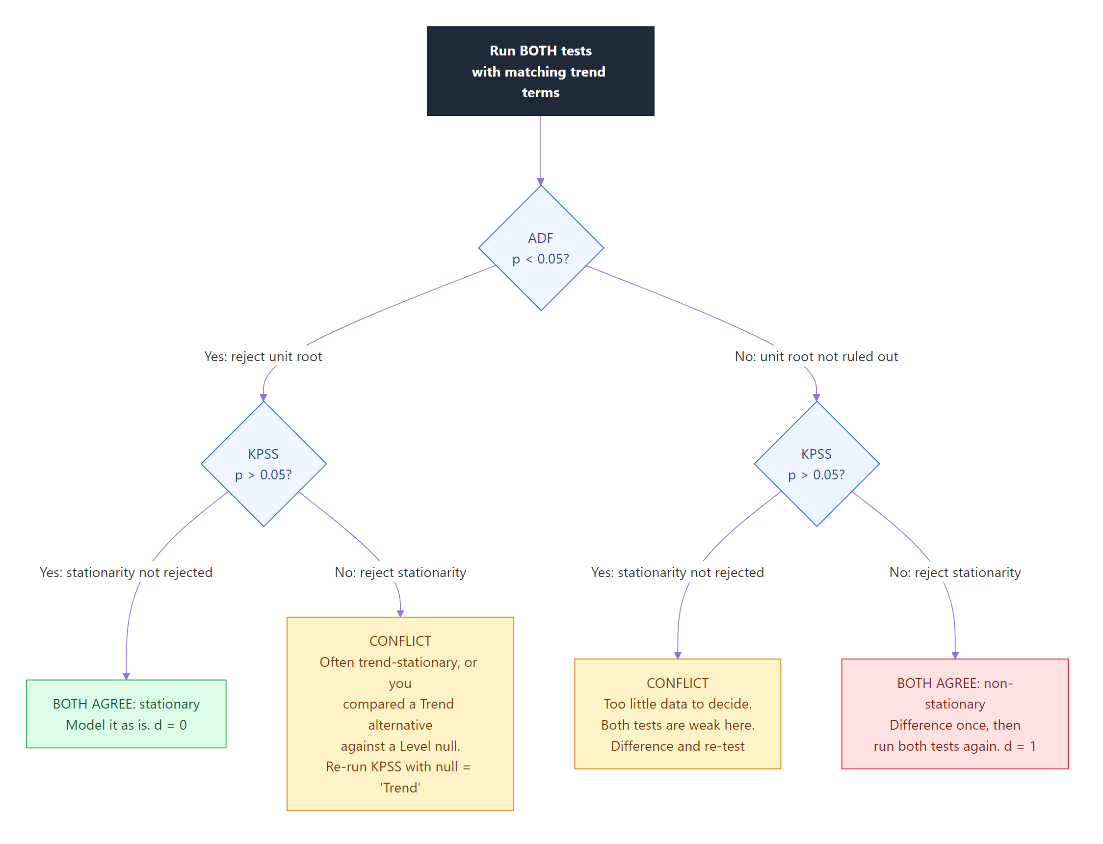
Figure 1: How to combine the two verdicts. The two cells on the outside are agreement. The two in the middle are the informative cases: a conflict is a message, not a malfunction.
The diagram gives you the full rule. In words:
| ADF | KPSS | What it means | What to do |
|---|---|---|---|
| p < 0.05 (reject unit root) | p > 0.05 (keep stationarity) | Both say stationary | Model it as is. d = 0 |
| p > 0.05 (keep unit root) | p < 0.05 (reject stationarity) | Both say non-stationary | Difference it. d = 1 |
| p < 0.05 (reject unit root) | p < 0.05 (reject stationarity) | Often trend-stationary, or mismatched trend terms | Re-run KPSS with null = "Trend". This was our case |
| p > 0.05 (keep unit root) | p > 0.05 (keep stationarity) | Neither test can decide | Not enough data. Difference and re-test |
The bottom-right case deserves a word, because it surprises people. Both tests failing to reject is not "doubly stationary". ADF failing to reject means "cannot rule out a unit root" and KPSS failing to reject means "cannot rule out stationarity", so both together mean the data is too short or too noisy to distinguish the two. That is a statement about your sample, not your series.
How many differences does your series need?
We now know AirPassengers has a trend. There are two ways to remove a trend, and which one is right depends on what kind of trend it is.
- A deterministic trend is an underlying line with noise around it. The cure is to subtract the line, called detrending.
- A stochastic trend is accumulated shocks, a unit root. The cure is differencing: model the changes instead of the levels.
Differencing means replacing each value with the change from the previous value, \(\Delta y_t = y_t - y_{t-1}\). If the series is a random walk, \(y_t = y_{t-1} + \varepsilon_t\), then \(\Delta y_t = \varepsilon_t\), which is stationary. Differencing converts a random walk into pure noise, which is exactly why it is the standard fix. The number of times you difference is called \(d\).
You do not have to choose \(d\) by squinting at p-values. forecast::ndiffs() runs a stationarity test and reads the verdict; if the verdict is "not stationary" it differences the series, tests the result, and repeats until the verdict comes back stationary, then reports how many rounds it took. Its seasonal twin nsdiffs() does the same for a repeating cycle and reports \(D\).
Order matters, and it is the opposite of what most people try first. Deal with the seasonality before testing the level, because a strong annual cycle is exactly the kind of structure that confuses both ADF and KPSS.
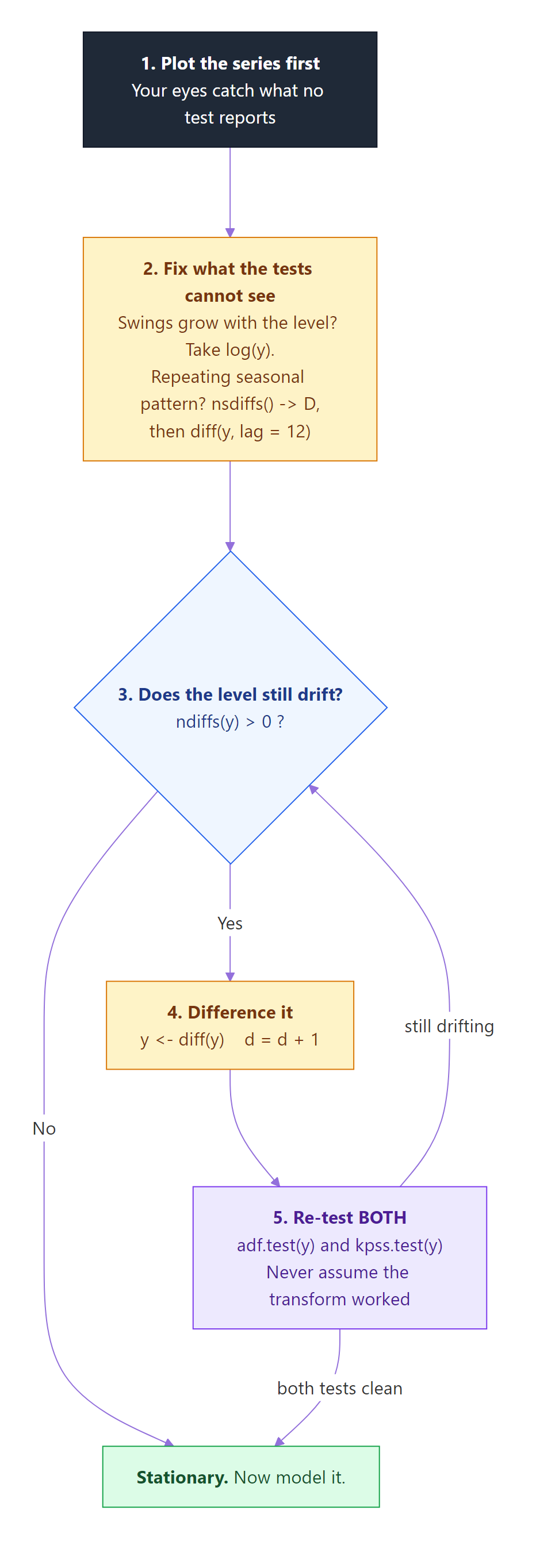
Figure 2: The order of operations. Fix what the tests cannot see (variance, seasonality) first, then test the level, then re-test after every transform.
All three answers agree: one seasonal difference and one ordinary difference. The fact that ndiffs() gives 1 whether it asks KPSS or ADF is reassuring; when those two disagree, you are in one of the middle rows of the table above and should look closer.
Differencing itself is diff(), and it is worth seeing exactly what it does to your data before trusting it.
Look at the two head() outputs together and the arithmetic is plain. January 1949 was 112 and February was 118, so February's differenced value is 118 - 112 = 6. March was 132, so its value is 132 - 118 = 14. April dropped to 129, giving 129 - 132 = -3. The series now describes change in passengers per month rather than passengers.
Notice you lost one observation (144 became 143) and January 1949 is gone. That is unavoidable: the first month has no previous month to subtract. Every difference costs you one point at the front, and a seasonal difference at lag 12 costs you twelve.
Did the differencing actually work?
Never assume a transform worked. Test it. This is the step people skip, and it is the step that catches the interesting problems.
Both tests now agree, and this time on a flat-line null. ADF rejects the unit root (p = 0.01) and KPSS does not reject level stationarity (its statistic fell from 2.7395 to a minuscule 0.014626, p = 0.1). By the top-left row of our table, that is the clean "both say stationary" verdict. Differencing worked.
Except it did not, quite. And no test on this page is going to tell you.
The tests are blind to variance
Remember rule 2 from the definition: constant variance. Both ADF and KPSS are built around the mean and the level. Neither one is checking whether the wobble is growing. So let us check it ourselves, the same way we did at the start.
The month-to-month changes swing more than twice as hard in the second half (standard deviation 43.7) as in the first (19.2). That violates rule 2 outright. Both tests just handed this series a clean bill of health, and both were wrong, because neither was looking at variance. This is the most important practical limitation on the page.
The cause is that airline traffic grows multiplicatively. A busy month in 1960 is not "50 thousand more" than a quiet one, it is "30 percent more", and 30 percent of a big number is a big number. The fix is to take logs first. Logs turn multiplicative behaviour into additive behaviour, because a constant percentage change becomes a constant additive change in log units.
There it is. On the log scale the two halves wobble by 0.1034 and 0.1103, which is as close to constant variance as real data gets. The 2.3-fold blowup is gone. Nothing about the differencing changed; only the scale did.
Note: No stationarity test asked you to take that log, and none would have complained if you had not. Deciding on a variance-stabilising transform is your job, done by eye on the plot, before the tests get involved. That is why the workflow starts with "plot it".
The full recipe
Now put the steps in the right order: log first, then seasonal difference, then ordinary difference, testing as we go.
diff(lap, lag = 12) subtracts each month's value from the same month one year earlier, which removes the annual cycle: it compares July with last July instead of with June. After that, ndiffs() still wants one ordinary difference for the remaining drift, so we apply it. The 13 lost observations are exactly the price we predicted: 12 for the seasonal difference and 1 for the ordinary one.
The final verdict.
ADF rejects the unit root (p = 0.01) and KPSS does not reject level stationarity (p = 0.1). Both agree, on a flat-line null, on a series whose variance we verified is stable. That is a genuinely stationary series, and log, d = 1, D = 1 is the recipe that got us there. It is also, not coincidentally, exactly the transformation behind the classic "airline model" that Box and Jenkins fitted to this very dataset.
Compare this picture with the one from section 2. The climb is gone, the annual saw-tooth is gone, and the teeth no longer grow. What is left is a band of wobble sitting flat around the red zero line, looking about the same in 1949 as in 1960. That is what stationary looks like, and it is what your ARIMA model wants.
When do these tests mislead you?
You have the recipe. Now here is when to distrust it, because every one of these will happen to you.
A trend does not always mean "difference it"
Not every trending series has a unit root. Build one that has a real straight-line trend and nothing else: no accumulation, no wandering, just a line plus independent noise.
That is the same "contradiction" as section 1, and now you know exactly what it is: ADF rejects the unit root (correct, there isn't one), and level-KPSS rejects flatness (correct, it slopes upward). This series is trend-stationary: stationary once you account for the line. It does not need differencing, it needs detrending.
Look closely at those two statistics: 0.04317 and 0.04317. Identical. That is not a coincidence, it is the definition. Running kpss.test(x, null = "Trend") and running level-KPSS on the residuals of lm(x ~ t) are the same computation. Seeing the two match is the clearest possible proof of what the null = "Trend" argument actually does: it regresses out a straight line and tests what remains.
The practical distinction: difference a trend-stationary series and you add noise you did not need; detrend a difference-stationary series and the trend you removed was never really there. On short, seasonal, real-world data the tests often cannot separate the two confidently, which is why forecasters usually prefer differencing: it handles both a stochastic trend and a slowly changing deterministic one, at the cost of a little efficiency.
The tests are weak on short series
ADF has low statistical power, which is jargon for "it often fails to reject even when it should". It is worst exactly when \(\phi\) is close to but below 1, because such a series looks a lot like a random walk over a short window.
arima.sim(model = list(ar = 0.95)) generates the AR(1) from section 3 with \(\phi = 0.95\). Since 0.95 is less than 1, this series is stationary, by construction, with certainty. ADF returned p = 0.5303 and failed to reject the unit root. The test is simply wrong here. Give it the identical process with more data and it recovers.
Same \(\phi\), same seed, 600 points instead of 60, and now p = 0.01. Nothing about the process changed; only the evidence did. Treat "ADF failed to reject" on a short series as "this test learned nothing", not as "there is a unit root".
Differencing more is not safer
Since differencing fixes non-stationarity, it is tempting to difference again for good measure. Do not. Differencing an already-stationary series (called over-differencing) injects artificial negative autocorrelation and inflates the variance your model has to explain.
ndiffs() correctly says white_noise needs zero differences. Difference it anyway and the standard deviation goes up, from 0.975 to 1.383, a factor of about 1.41. That number is not random: differencing two independent draws each with variance \(\sigma^2\) gives a result with variance \(2\sigma^2\), and \(\sqrt{2} \approx 1.414\). You took a clean series and made it noisier. Trust ndiffs(), and stop when it says stop.
FAQ
Should I use ADF or KPSS? Both, always, and compare them with the table in section 6. They have opposite nulls, so each covers the other's blind spot: ADF cannot confirm stationarity (it can only fail to reject a unit root) and KPSS cannot confirm a unit root. Running one alone throws away half the information.
My ADF p-value is 0.01 but KPSS says non-stationary. Which do I believe? Neither is wrong: you are comparing a trend-aware alternative against a flat-line null, exactly as in section 1. Re-run KPSS with null = "Trend". If it stops rejecting, your series is trend-stationary and the two tests agree.
What about the Phillips-Perron test? pp.test() in tseries is a third unit-root test with the same null as ADF, so you read its p-value the same way. The difference is only in how it handles autocorrelation: where ADF adds lagged change terms to the regression, Phillips-Perron fits the plain regression and then corrects the test statistic afterwards. It usually agrees with ADF, and when it does not, you are typically in the low-power situation described above, where neither test is telling you much. ADF plus KPSS already covers both directions, so adding a third test rarely changes the decision.
Why does R warn "p-value smaller than printed p-value"? Both tests interpolate p-values from a small printed table (roughly 0.01 to 0.99 for ADF, 0.01 to 0.1 for KPSS). When your statistic falls off the end, R returns the nearest edge value and warns you the truth is more extreme. It is a table limit, not an error, and p = 0.01 should be read as "0.01 or less".
Do I need to test for stationarity if I use auto.arima()? Not manually, because auto.arima() calls ndiffs() and nsdiffs() internally to pick \(d\) and \(D\). But you should still plot the series and decide on a log or other variance-stabilising transform yourself, because no part of that automatic machinery checks whether your variance is growing.
How many differences is too many? More than two ordinary differences (\(d > 2\)) or more than one seasonal difference (\(D > 1\)) is almost always a sign that something else is wrong, usually a variance problem that a log would fix. If ndiffs() keeps asking for more, go back and plot the series.
Does a stationarity test check seasonality? Not usefully. Strong seasonality violates rule 3 and confuses both tests, which is why the workflow removes it with nsdiffs() and diff(y, lag = 12) before testing the level. Use nsdiffs() for the seasonal question and ndiffs() for the level question.
Summary
We started with AirPassengers and two tests that appeared to contradict each other. They did not: adf.test() always fits a trend, kpss.test() defaults to a flat line, and once we asked both the same question (null = "Trend", p = 0.1) they agreed the series has a trend but no random walk. Taking logs stabilised the variance that neither test could see, one seasonal difference removed the annual cycle, one ordinary difference removed the drift, and the fully transformed series passed both tests on a flat-line null. That is the airline model's recipe, derived from evidence rather than assumed.
| Idea | What to remember |
|---|---|
| Stationary | Constant mean, constant variance, autocovariance depending only on the gap |
| Unit root | \(\phi = 1\) in \(y_t = \phi y_{t-1} + \varepsilon_t\); shocks never decay; a random walk |
adf.test() |
Null = has a unit root. Small p means stationary. Always fits a trend |
kpss.test() |
Null = is stationary. Small p means non-stationary. Default null is "Level" |
| The conflict case | Mismatched trend terms. Re-run KPSS with null = "Trend" |
ndiffs() / nsdiffs() |
Let them choose \(d\) and \(D\). Do the seasonal one first |
diff() |
Costs one observation per difference, twelve for a seasonal one |
| The blind spot | No test checks variance. Plot first; take logs if swings grow with the level |
| Low power | "ADF did not reject" on a short series means the test learned nothing |
| Over-differencing | Inflates variance by \(\sqrt{2}\) per needless difference. Stop when ndiffs() says 0 |
References
- Forecasting: Principles and Practice, "Stationarity and differencing" - Hyndman and Athanasopoulos. The canonical free treatment of everything on this page, and the source of the "difference first, ask questions later" workflow.
- Unit root tests - Rob Hyndman on why he prefers KPSS-based
ndiffs()over ADF for choosing \(d\). Short, opinionated, and from the author of theforecastpackage. - tseries reference manual - the definitive statement of what
adf.test()andkpss.test()actually fit, including the constant-and-trend regression and the interpolated p-value tables. - ndiffs() documentation - the exact algorithm behind the number of differences, and how to change the test or significance level.
- Kwiatkowski, Phillips, Schmidt and Shin (1992) - the original KPSS paper, which introduced the "null of stationarity" idea specifically to complement unit-root tests like ADF.
- urca reference manual - when you outgrow
tseriesand need to control the deterministic terms yourself,ur.df()andur.kpss()are the tools, with proper critical-value tables. - Forecasting: Principles and Practice, "Seasonal ARIMA models" - where \(d\) and \(D\) go once you have them, including the airline model this post reconstructed.
- CRAN Task View: Time Series Analysis - the maintained map of the R time series ecosystem, with a section on unit roots and cointegration.
Continue Learning
- Time Series Objects in R covers the
tsclass thatwindow(),diff()and both tests rely on, plus when to reach forxtsortsibbleinstead. - Visualize Time Series in R goes deeper on the "plot it first" step, which is where you catch the variance problems no test reports.
- EDA for Time Series in R puts stationarity testing in the wider set of checks to run before modelling.
- Time Series Exercises in R has practice problems if you want to drill differencing on other series.