Prediction Intervals in R: Quantify Forecast Uncertainty
A prediction interval is a range that a single future observation is expected to fall inside, with a stated probability. In R you get one from predict(model, newdata, interval = "prediction") for a regression and from forecast(model, h) for a time series, and it is always wider than a confidence interval because it carries two kinds of uncertainty instead of one.
What is a prediction interval, and why is a point forecast not enough?
A single predicted number carries no warning about how wrong it might be. It tells you roughly where the middle of the outcome sits, but nothing about how far reality could land from it. A prediction interval fixes that by reporting a range instead of a point. R hands you one from the same predict() call you already use, by adding a single argument.
Let's make that concrete with a model everybody can check. We will predict a car's fuel economy from its weight using mtcars, a dataset built into R with 32 cars, then ask what a brand new 3000 lb car would get.
The first line fits a straight line through the 32 cars, relating weight (wt, in thousands of pounds) to fuel economy (mpg). The second line builds a one-row data frame holding the car we want to predict for. The bare predict() call returns one number, 21.25. Adding interval = "prediction" returns three: the same 21.25 as fit, plus a lower bound lwr of 14.93 and an upper bound upr of 27.57.
Those two answers describe very different states of knowledge. The first says "21.25 mpg". The second says "somewhere between 14.9 and 27.6 mpg, and I am 95% confident about that range". If you were budgeting fuel for a fleet, the second answer is the one that keeps you out of trouble, because 14.9 is a plausible outcome and 21.25 is not a promise.
The level = 0.95 argument is what "95%" means here. Over many new cars, about 95 out of every 100 should land inside an interval built this way. That is the claim, and later in this tutorial we will actually test it rather than take it on faith.
The interval also moves as the input moves. Here are three cars of different weights, with the width of each interval shown alongside.
We built a three-row data frame of weights, asked for a prediction interval at each, then glued the inputs, the interval and its width into one table. cbind() joins columns side by side, and the width column is just upr minus lwr.
Two things stand out. The centre slides down as cars get heavier, from 26.6 mpg at 2000 lb to 15.9 mpg at 4000 lb, which is the regression line doing its job. The width barely moves, hovering near 12.6 to 12.9 mpg. That width is the real message of this page: no matter which car you ask about, your honest uncertainty about it spans roughly 13 mpg.
Try it: Predict the fuel economy of a heavy 4500 lb car, but at the 80% level instead of 95%. Before you run it, predict whether the interval will be wider or narrower than a 95% one.
Click to reveal solution
Explanation: The 80% interval spans 8.3 mpg, while the 95% interval for the same kind of car spans about 12.8 mpg. Demanding less confidence buys you a tighter range. You have not learned anything new about the car, you have simply agreed to be wrong more often.
What are the two sources of uncertainty behind a prediction?
The interval above was about 13 mpg wide, and that number came from somewhere. Understanding where is what separates people who copy interval = "prediction" from people who can defend the result in a meeting. There are exactly two ingredients, and we can measure both.
The first ingredient is that we do not know the true relationship between weight and mpg. We estimated a line from 32 cars, and a different 32 cars would have given a slightly different line. So the line itself wobbles.
The second ingredient is that even if somebody handed us the perfect true line, an individual car would still not sit exactly on it. Two identical 3000 lb cars have different engines and different tyres, so their mpg differs. That scatter never goes away, no matter how much data you collect.
Rather than assert this, let's measure the first ingredient. We will invent a world where we know the truth: outcomes follow y = 10 + 1.5x plus random noise with a standard deviation of 4. Then we will draw 500 separate datasets from that world, fit a line to each one, and watch where the fitted line lands at x = 10.
Inside the loop we generate 20 fresh observations, fit lm() to them, then evaluate the fitted line at x = 10. The expression coef(lm(y ~ x)) %*% c(1, 10) multiplies the intercept by 1 and the slope by 10, which is exactly the fitted value at that point. We store all 500 answers, then summarise them.
The true value at x = 10 is 10 + 1.5 * 10, which is 25. Our 500 fitted lines average 25.019, so the procedure is unbiased. But they scatter around it with a standard deviation of 0.860. That 0.860 is ingredient one, measured rather than assumed.
Now for the second ingredient. In this invented world we know the noise standard deviation is 4, because we put it there. Let's confirm that the two ingredients combine the way the theory claims, by drawing 500 actual new observations at x = 10 and comparing their spread to the combination.
We drew 500 genuine new observations, each one the true mean of 25 plus its own random noise. Then we lined up four numbers: the wobble of the line (0.860), the noise standard deviation (4), the two combined as sqrt(0.860^2 + 4^2) which gives 4.091, and the observed spread of the new points, 4.085.
The predicted 4.091 and the observed 4.085 agree to within a rounding error. Standard deviations do not add directly. They add as squares and then get square-rooted, which is what the block title means by adding in quadrature, and it is why the total is 4.09 rather than 4.86. Notice how lopsided the contributions are: the noise term of 4 dominates the line wobble of 0.86 almost completely.
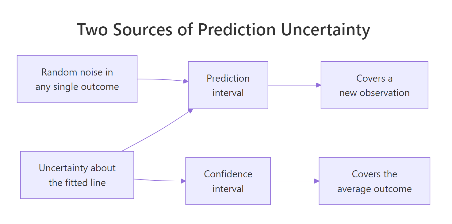
Figure 1: A confidence interval carries only the uncertainty about the fitted line, while a prediction interval carries that plus the noise in any single outcome.
Now that the simulation has made the point, the formula is just bookkeeping. For a simple regression, the standard error used to build a prediction interval at a new input $x_0$ is:
$$\text{SE}_{\text{pred}} = \hat{\sigma}\sqrt{1 + \frac{1}{n} + \frac{(x_0 - \bar{x})^2}{\sum_{i=1}^{n}(x_i - \bar{x})^2}}$$
Where:
- $\hat{\sigma}$ = the estimated standard deviation of the residuals, R's "residual standard error"
- $n$ = the number of observations used to fit the model
- $x_0$ = the input value you are predicting at
- $\bar{x}$ = the mean of the inputs in the training data
Read the three terms under the square root as a story. The 1 is the irreducible noise in a single outcome, ingredient two. The 1/n shrinks as you gather more data, because a bigger sample pins down the line better. The last term, called the leverage term, grows as $x_0$ moves away from the centre of your data, because a line pivots around its middle and the far ends swing most.
That 1 is the reason a prediction interval never collapses to zero. Collect a million cars and the last two terms vanish, but the 1 stays, and with it the noise of an individual car.
You do not have to trust predict() on this. Let's rebuild the exact interval from the first code block by hand, using only the formula and qt() for the t-distribution multiplier.
We pulled the residual standard error out of summary(model), counted the 32 rows, then plugged the weights into the formula. qt(0.975, df = 30) gives the multiplier that puts 95% of a t-distribution between plus and minus itself, leaving 2.5% in each tail. The interval is then the point estimate plus or minus that multiplier times se_pred.
The result, 14.930 to 27.574, is identical to what predict() returned at the top of this page. The function is not doing anything mysterious. Also note how close se_pred (3.095) sits to sigma_hat (3.046): the noise term contributes nearly all of it, exactly as the simulation showed.
Try it: The mean car weight in mtcars is about 3.22. Build prediction intervals at a weight near that centre (3.2) and at a weight well beyond the heaviest cars in the data (5.4), then compare the widths.
Click to reveal solution
Explanation: The interval widens from 12.63 to 13.58 as you move out to a weight heavier than any car in the training data. The model still gives you an answer at wt = 5.4, and it widens the interval a little to admit extra doubt, but it cannot warn you that the straight-line relationship may not hold out there at all. That risk is invisible to the formula.
How does a prediction interval differ from a confidence interval?
Both intervals come from the same predict() call and differ by one word, so they get mixed up constantly. They answer genuinely different questions, and picking the wrong one is the single most common mistake in this whole area.
A confidence interval answers: "Where is the average mpg of all 3000 lb cars?" A prediction interval answers: "What will this particular 3000 lb car get?" The first is about a population average, which is a fixed quantity we are trying to pin down. The second is about one random outcome, which has its own noise on top.
Let's put them next to each other for the same car.
We asked for both interval types at the same input, pulled out the fit and the two bounds from each, then assembled them into a small comparison table. Indexing a predict() result with [1], [2] and [3] grabs the fit, the lower bound and the upper bound in order.
Both intervals share the same centre of 21.25, because they use the same fitted line. But the confidence interval spans 2.25 mpg while the prediction interval spans 12.64 mpg, which is 5.6 times wider. That ratio is the noise term overwhelming the line wobble, the same lopsidedness we measured in the previous section.
interval = "confidence", and if it is about one specific case somebody is about to buy or budget for, ask for interval = "prediction".Here is where most tutorials stop. We are going to test the claim instead, because the difference between these two intervals is not a matter of taste. One of them is simply wrong for predicting a single outcome, and we can measure how wrong.
The experiment: run 4000 miniature studies. In each one, generate 20 observations from a known truth, fit a model, then build both intervals at x = 10.
Then check three things in every study. Does the confidence interval contain the true mean of 25? Does it contain a genuinely new observation? Does the prediction interval contain that new observation?
Each pass through the loop is one complete study: draw data, fit a model, build both intervals, then draw one honest new observation np from the same true world. The three hits columns record whether each target landed inside its interval. Taking colMeans() of a logical matrix converts those TRUE and FALSE values into proportions.
Read those three numbers carefully, because they are the heart of this section.
The confidence interval captured the true mean 95.3% of the time. It is doing its job perfectly, and a 95% confidence interval is genuinely a 95% confidence interval. The prediction interval captured a new observation 95.2% of the time. Also doing its job perfectly.
But the confidence interval captured a new observation only 34.2% of the time. If you report a confidence interval to somebody who is asking about one future case, you will be wrong roughly two times in three while claiming to be wrong one time in twenty.
Seeing the two bands drawn over the actual data makes the distinction hard to forget. The plot below draws the prediction band as the pale outer ribbon and the confidence band as the darker inner ribbon, with the 32 real cars on top.
We built a fine grid of 100 weights spanning the data, computed both intervals across the whole grid, then bundled everything into one data frame so ggplot2 can draw it. Each geom_ribbon() shades the area between a lower and upper bound, and drawing the prediction ribbon first puts the narrower confidence ribbon on top of it.
Look at where the real cars sit. Almost all of them fall inside the pale prediction band, which is precisely what a 95% prediction interval promises. Most of them fall outside the darker confidence band, and that is not a failure. The confidence band was never claiming to contain individual cars, only the average car at each weight.
Try it: Compute the width of both intervals for a light 2000 lb car, and work out how many times wider the prediction interval is.
Click to reveal solution
Explanation: The ratio is 3.65 here versus 5.6 at wt = 3.0. The gap between the two intervals shrinks as you move away from the centre of the data, because the confidence interval is the part that grows with distance while the noise term stays constant.
How do you get prediction intervals for a time series forecast?
Everything so far used a regression, where a prediction interval attaches to a value of x. Forecasting works the same way, except the thing you are predicting at is a future time period, and you usually want a whole run of them. The forecast package builds the intervals for you and returns them alongside the point forecast.
We will use AirPassengers, a built-in series of monthly international airline passengers from 1949 to 1960, in thousands. It trends upward and has a strong yearly cycle, which makes it a realistic test. The ets() function fits an exponential smoothing model, choosing the trend and seasonal form automatically.
ets() fits the model to the whole series. forecast(fit_air, h = 12) projects 12 months past the end of the data, which takes us through 1961. Converting the result with as.data.frame() turns it into a readable table, and head(..., 4) shows the first four months.
Every row carries five numbers instead of one. For January 1961 the point forecast is 441.8 thousand passengers. The 80% interval runs from 419.6 to 464.0, and the 95% interval runs wider, from 407.9 to 475.7. Two levels come back by default because they answer different appetites for risk: the 80% range is the "likely" case and the 95% range is the "plan for it" case.
The 95% interval nests around the 80% one, which it must. Asking for more confidence can only ever mean accepting a wider range, and you can read that directly off the columns.
A fan chart shows the same information as a picture, with the shading getting lighter as confidence widens.
autoplot() knows how to draw a forecast object, so it plots the historical series, the point forecast continuing from the end of it, and the two interval bands as nested shaded regions. The dark inner band is the 80% interval and the pale outer band is the 95% one.
The shape it draws is the whole story of forecast uncertainty. Historical data is a single line, because it already happened. The forecast is a widening cone, because the future has not. The further ahead you look, the wider the range of outcomes the model treats as plausible.
level = c(50, 95) to forecast() gives you a median-ish range and a planning range instead of the default 80 and 95, and passing a single number like level = 90 returns just one pair of bounds.Try it: Forecast 24 months ahead at the 90% level, then look at the final two rows to see how much the model is willing to commit to two years out.
Click to reveal solution
Explanation: Two years out, the 90% interval for December 1962 runs from 332 to 599 thousand passengers. That is a range of 266, against 68 for January 1961 at the even wider 95% level, so the interval is close to four times as wide two years out. You still get a point forecast that far ahead, and the width is what tells you how much it is worth.
Why do forecast intervals get wider the further ahead you look?
That widening cone is not decoration, and it is not the model getting worse. It follows from a simple mechanical fact: to forecast two steps ahead, you have to stand on your one-step-ahead forecast. If step one was wrong, step two inherits that error and adds its own on top.
Think of walking in fog. After one step you might be a metre off course. After two steps you are off by that first metre plus whatever the second step adds, and errors keep piling up rather than cancelling. The spread of where you might be grows with every step.

Figure 2: Each forecast step inherits the error of every step before it, so the spread of possible outcomes grows with the horizon.
Let's watch it happen in the airline forecast we already built, by extracting the 95% interval width at each of the 12 horizons.
A forecast object stores its bounds in matrices called $lower and $upper, with one column per confidence level. We pulled the "95%" column from each, subtracted to get widths, then expressed every width as a multiple of the first one.
The overall climb is clear: by horizon 8 the interval is 3.16 times wider than at horizon 1. But the path is bumpy, dipping at horizons 9 through 11 before rising again. That wobble is worth explaining rather than glossing over.
This model is multiplicative and seasonal, so the interval width scales with the seasonal level being forecast. Summer months carry more traffic and therefore more absolute uncertainty than winter months, and that seasonal shape rides on top of the underlying growth.
To see the pure accumulation effect without seasonality confusing it, we need a simpler series. A random walk is the cleanest possible case: each value is the previous value plus a random shock. The naive() method forecasts it by carrying the last value forward.
We built a 150-point random walk by running cumsum() over random shocks, wrapped it in ts() so the forecasting functions treat it as a time series, forecast 8 steps with naive(), then compared the width ratio against the square root of the horizon.
The ratio and sqrt_h columns match to three decimal places at every horizon. This is not an approximation that happens to look close. For a random walk the h-step forecast error is the sum of h independent shocks, and the standard deviation of that sum is exactly $\sigma\sqrt{h}$.
Why a square root rather than plain multiplication? Because independent errors partly cancel. Some shocks push up and some push down, so h shocks do not give you h times the spread. Let's confirm the mechanism directly by simulating the accumulation.
For each horizon from 1 to 6, we simulated 4000 futures. Each future is the sum of h independent shocks, exactly what accumulates between now and horizon h. Then we took the standard deviation across those 4000 futures and set it beside the theoretical $\sigma\sqrt{h}$.
The simulated column tracks the theory column closely at every horizon, with small gaps that are just Monte Carlo sampling error from using 4000 draws instead of infinitely many. Nothing was assumed here: we added up random shocks and the square root fell out on its own.
Try it: Using the same walk series, forecast 16 steps ahead and confirm that the width at horizon 16 is exactly 4 times the width at horizon 1.
Click to reveal solution
Explanation: Sixteen times the horizon buys only four times the uncertainty, because $\sqrt{16} = 4$. This is genuinely good news for forecasters. Uncertainty grows steadily rather than explosively, which is why medium-range forecasts remain useful at all.
What do you do when the residuals are not normal?
Every interval so far rested on an assumption we have not examined: that the model's errors follow a normal distribution, the symmetric bell curve. That is what justifies putting the same distance above and below the point forecast. When the errors are lopsided, a symmetric interval is the wrong shape, and it will be wrong in a specific direction.
Residuals are the leftovers: actual value minus what the model predicted, for every period in the training data. They are our only evidence about the shape of future errors, so checking them is not optional.
Let's build a series that deliberately breaks the assumption. Its shocks come from an exponential distribution, which can produce large positive jumps but never large negative ones.
We generated the series, fitted naive() to it, then pulled the residuals with residuals(). na.omit() drops the first one, which is missing because a naive forecast has nothing to stand on at period 1. Then we computed three diagnostics and ran a formal normality test.
The mean is 0.108 but the median is negative at -0.422. For a symmetric distribution those two would be close together, so the gap alone is a warning. The skewness statistic of 2.243 confirms it: zero means symmetric, and anything past about 1 means clearly lopsided to the right. The Shapiro-Wilk test returns a p-value of 1.827e-13, which is a decisive rejection of normality.
The fix is to stop assuming a shape and use the shape the data actually shows. That is what the bootstrap does. Instead of multiplying a standard error by a normal quantile, it resamples the observed residuals at random, adds them to the forecast path thousands of times, and reads the interval bounds straight off the resulting spread of simulated futures.
We forecast the same series twice. The only difference is bootstrap = TRUE, which tells naive() to simulate npaths = 5000 future paths by resampling the actual residuals instead of assuming a bell curve. Because the simulation is random, set.seed(31) makes the result reproducible.
Compare the two pairs of bounds at any horizon. At horizon 4 the normal interval runs 107.43 to 124.10, centred on the point forecast of 115.76. The bootstrap interval runs 109.81 to 126.52, which is shifted upward and no longer centred. The residuals it resampled contain more large upward values than large downward ones, so both simulated bounds sit higher than the symmetric ones.
That asymmetry is the point. The normal interval is not merely a bit too narrow or too wide, it is the wrong shape: it leaves as much room below the forecast as above it, in a series whose errors are far larger on the upside.
A related situation produces asymmetric intervals for a completely different reason. If you fit a model on a transformed scale, such as logs, and then convert back to the original units, the interval comes back lopsided even when the errors were perfectly normal on the log scale.
Setting lambda = 0 tells the forecast package to fit on the log scale and automatically convert the results back to passenger counts. The below and above columns measure how far the interval reaches on each side of the point forecast.
They never match. In June 1961 the interval reaches 75.6 below the point forecast but 87.0 above it. That is correct, not a bug.
A symmetric interval on the log scale becomes a lopsided one after exponentiating, because the exponential function stretches the upper half more than the lower half. It also guarantees the lower bound stays positive, which matters when the quantity being forecast cannot go below zero.
Try it: Measure the asymmetry directly. Using fc_normal and fc_boot from above, compute how far each interval reaches below and above the point forecast at horizon 4.
Click to reveal solution
Explanation: The normal interval is symmetric to the penny, 8.33 in each direction, because that is what the method forces. The bootstrap reaches only 5.96 below but 10.76 above, nearly twice as far up as down. It changed the interval's shape, not just its width, which is something no multiplier on a standard error can ever do.
How do you check whether your prediction intervals are honest?
A 95% prediction interval makes a testable claim: about 95% of actual outcomes should land inside intervals built this way. Almost nobody tests it. This section is the one that separates a forecast you can defend from a forecast you merely produced.
The test is simple. Hide the end of your series from the model, forecast that hidden stretch, then count how many actual values landed inside the interval. If a 95% interval only catches 70% of them, your interval is too narrow and you now know it before your stakeholders find out the hard way.
Let's split AirPassengers, training on everything through 1958 and holding back the final two years.
window() slices a time series by date rather than by row number, taking c(year, month) pairs. We kept 120 months for training and set aside the last 24, which the model will never see.
Now fit on the training portion only, forecast the 24 held-out months, and count the hits.
We fitted ets() to the training months alone, forecast 24 steps at both confidence levels, then built two logical vectors marking whether each actual value fell between its bounds. mean() of a logical vector gives the proportion of TRUE values, which is exactly the observed coverage. The nominal_ numbers are the coverage we asked for, and the actual_ numbers are the coverage we got.
The results are uncomfortable, and that is why they are worth showing. The 80% interval was supposed to catch about 19 of the 24 months, and it caught 7. The 95% interval was supposed to catch roughly 23, and it caught 21.
Both intervals are too narrow, and there are real reasons for that. The interval only accounts for random noise around the fitted model. It does not account for the model being slightly the wrong shape, nor for the growth pattern in 1959 and 1960 running a little differently from the 1949 to 1958 stretch the model learned on. Nothing in the arithmetic can price in "my model is not quite right", and in practice that is often the largest source of forecast error.
Coverage is only half the story, though. An interval from zero to infinity would cover 100% of outcomes and be completely useless, so width has to be read alongside it.
We averaged the 95% interval width across all 24 test months, compared it against the average passenger count over the same period, and expressed the width as a percentage of that level.
The average 95% interval spans 173 thousand passengers against an average level of 452 thousand, so it is 38% as wide as the thing being forecast. Judge that against your decision. Booking crew rosters within a 38% band is probably workable; committing to aircraft purchases on it is not. A good forecast report gives both numbers, because coverage without width flatters the model and width without coverage is meaningless.
Try it: Coverage usually decays as the horizon grows. Check the 95% coverage over just the first test year, 1959, and compare it against the 87.5% across both years.
Click to reveal solution
Explanation: The first year alone covered 83.3%, slightly below the 87.5% across both years. Coverage does not decay uniformly here because the interval widens with horizon at the same time as the errors grow, so the two effects partly offset. What matters is that both numbers sit under the promised 95%, so the shortfall is a property of the model rather than a fluke of one year.
Complete Example
Let's run the whole workflow once, start to finish, on a series we have not touched. USAccDeaths records monthly accidental deaths in the United States from 1973 to 1978. We will train on everything up to the end of 1977, forecast all of 1978 with a 95% interval, then check the interval against what actually happened.
We held back 1978, fitted ets() on the five preceding years, then forecast 12 months at a single 95% level. January 1978 comes out at 7948 deaths with an interval from 7388 to 8509, a range of about 1100.
Now the part that most workflows skip. Did those intervals actually contain what happened?
We compared every 1978 actual against its bounds, then reported four numbers: how many months landed inside, the coverage proportion, the average interval width, and that width as a share of the average monthly death count.
All 12 months landed inside, giving 100% coverage against a promised 95%. The average width is 2036 deaths, which is 23% of the typical monthly level. Both numbers are healthier than the airline case: better coverage on a proportionally tighter interval.
The contrast is the lesson. The same ets() function with the same 95% setting under-covered badly on AirPassengers and covered fully on USAccDeaths. Coverage is a property of a specific model paired with a specific series, never a guarantee that ships with the function, which is exactly why you test it every time.
Finally, draw the forecast with the truth laid over the top.
autoplot() draws the history, the point forecast and the shaded interval, then autolayer() adds the held-out 1978 actuals as a separate coloured line on top. This single picture is the most honest forecast report you can hand somebody: here is what I predicted, here is the range I claimed, here is what happened.
Every 1978 point tracks inside the band, and the seasonal dip and summer peak both land where the model expected. When a chart looks like this, the interval earned its keep.
Practice Exercises
Exercise 1: Prediction intervals across a predictor range
Fit a model predicting mpg from hp (horsepower) in mtcars, then produce 90% prediction intervals at hp values of 100, 150 and 200. Add a width column and work out which of the three is narrowest, then explain why.
Click to reveal solution
Explanation: The hp = 150 interval is narrowest at 13.32, because the mean horsepower in mtcars is about 147 and the leverage term in the standard error formula is smallest at the centre of the data. The differences are tiny, though, since the irreducible noise term dominates all three, which is the same pattern you saw with car weight.
Exercise 2: Pick a model on coverage and width together
Hold out 1977 from USAccDeaths and train on everything before it. Forecast 1977 twice, once with ets() and once with snaive() (the seasonal naive method, which simply repeats last year's value). Score both on 95% coverage and mean interval width, then decide which model you would ship.
Click to reveal solution
Explanation: Both methods covered all 12 months, so coverage cannot separate them. Width can: ets() delivers the same coverage in a band that is about 300 deaths narrower every month. When two models are equally honest, the more precise one wins, and this is exactly why you report both numbers rather than coverage alone.
Exercise 3: Prove the coverage claim is literal
A 50% prediction interval sounds almost useless, but it makes a precise claim: half of new observations should land inside it. Test that claim by simulation. Generate 3000 small datasets from y = 3 + 2x with noise of sd 5, build a 50% prediction interval at x = 8 each time, and check how often a genuinely new observation falls inside.
Click to reveal solution
Explanation: Observed coverage is 0.502 against a nominal 0.500. The claim is exactly as literal as it sounds. This also shows what "correct" looks like, which is the yardstick you hold your real forecasts against when their measured coverage comes back at 0.29.
Frequently asked questions
Is a prediction interval the same as a confidence interval?
No, and the gap is large. A confidence interval covers the average outcome at a given input, while a prediction interval covers a single new outcome. In the 4000-run simulation on this page, a 95% confidence interval contained the next observation only 34.2% of the time, so the two are not interchangeable.
Why is my prediction interval so wide?
Because it carries irreducible noise, the variation between individual outcomes that no model can explain. That term does not shrink with more data. If your interval is wider than you can act on, the fix is a better model with genuinely informative predictors, not a narrower interval.
Can I make the interval narrower?
Three honest routes exist. Lower the confidence level, which trades coverage for tightness. Improve the model so that less variation is left unexplained. Collect more data, which shrinks the parameter-uncertainty terms but never the noise term.
Anything else is just relabelling the same uncertainty. A narrower interval that you did not earn is simply a wrong interval.
Do prediction intervals require normally distributed data?
They require roughly normal residuals, not normal data. Check with a residual plot or shapiro.test(). If the residuals are skewed, pass bootstrap = TRUE to forecast() or naive() and the interval will be built from the residuals' actual shape instead.
Why does the interval widen when I predict far outside my data range?
The leverage term in the standard error formula grows with the squared distance from the mean of your predictor. Be careful, though: that widening only prices in extra statistical noise, not the possibility that the relationship changes shape entirely outside the range you observed. Extrapolation is riskier than the interval admits.
Which R functions give prediction intervals?
predict() with interval = "prediction" covers lm and glm style models. forecast() from the forecast package returns them for time series models such as ets() and arima(). The tidyverts fable package produces full forecast distributions from which any interval can be extracted.
Summary
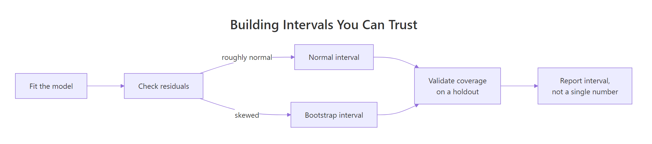
Figure 3: The full path from a fitted model to a prediction interval you can defend.
| Idea | What to remember |
|---|---|
| What it is | A range a single future observation should fall inside, with a stated probability |
| Two sources | Uncertainty about the fitted line, plus irreducible noise in any individual outcome |
| vs confidence interval | A confidence interval covers the average outcome, and caught a new observation only 34.2% of the time in simulation |
| For a regression | predict(model, newdata, interval = "prediction", level = 0.95) |
| For a forecast | forecast(model, h) returns 80% and 95% bounds in $lower and $upper |
| Why it widens | Each step inherits earlier errors; for a random walk the width grows exactly as the square root of the horizon |
| When residuals are skewed | Use bootstrap = TRUE so the interval takes its shape from the real residuals |
| Transformed models | Back-transformed intervals are asymmetric by design, and that is correct |
| Always do this | Test coverage on held-out data, and report interval width beside it |
The habit worth taking away is small and cheap. Whenever you produce a forecast, produce its interval, then check on held-out data whether that interval kept its promise. A point forecast that turns out wrong damages your credibility. An interval that was honest about its own uncertainty, even a wide one, protects it.
References
- Hyndman, R.J. & Athanasopoulos, G. Forecasting: Principles and Practice, 3rd edition. Section 5.5, Distributional forecasts and prediction intervals. Link
- Hyndman, R.J. & Athanasopoulos, G. Forecasting: Principles and Practice, 3rd edition. Section 3.1, Transformations and adjustments (back-transformed intervals). Link
- R Core Team.
predict.lmdocumentation, the source ofinterval = "prediction". Link - Hyndman, R.J.
forecastpackage reference,forecast.ets. Link - Hyndman, R.J. & Khandakar, Y. (2008). Automatic Time Series Forecasting: The forecast Package for R. Journal of Statistical Software, 27(3). Link
forecastpackage on CRAN. Link- R Core Team. An Introduction to R, the reference for
lm()and model formulas. Link fablepackage documentation, distributional forecasting in the tidyverts framework. Link
Continue Learning
- Forecast Accuracy in R scores how close your point forecasts land, which is the natural companion to knowing how uncertain they are.
- ETS Models in R explains the exponential smoothing models that produced every forecast interval on this page.
- Confidence Intervals in R goes deep on the other interval, the one that covers an average rather than a single outcome.
- Time Series Cross-Validation in R validates a model across many forecast origins instead of the single holdout used here.